Getting started
Trying it out
While we consider pyMOR mainly as a library for building MOR applications, we
ship a few example scripts. These can be found in the src/pymordemos
directory of the source repository (some are available as Jupyter notebooks in
the notebooks directory). Try launching one of them using the pymor-demo
script:
pymor-demo thermalblock --plot-err --plot-solutions 3 2 3 32
The demo scripts can also be launched directly from the source tree:
./thermalblock.py --plot-err --plot-solutions 3 2 3 32
This will reduce the so called thermal block problem using the reduced basis method with a greedy basis generation algorithm. The thermal block problem consists in solving the stationary heat equation
- ∇ ⋅ [ d(x, μ) ∇ u(x, μ) ] = 1     for x in Ω
                  u(x, μ)   = 0     for x in ∂Ω
on the domain Ω = [0,1]^2 for the unknown u. The domain is partitioned into
XBLOCKS x YBLOCKS blocks (XBLOCKS and YBLOCKS are the first
two arguments to thermalblock.py). The thermal conductivity d(x, μ)
is constant on each block (i,j) with value μ_ij:
(0,1)------------------(1,1)
|        |        |        |
|  μ_11  |  μ_12  |  μ_13  |
|        |        |        |
|---------------------------
|        |        |        |
|  μ_21  |  μ_22  |  μ_23  |
|        |        |        |
(0,0)------------------(1,0)
The real numbers μ_ij form the XBLOCKS x YBLOCKS - dimensional parameter
on which the solution depends.
Running thermalblock.py will first produce plots of two detailed
solutions of the problem for different randomly chosen parameters
using linear finite elements. (The size of the grid can be controlled
via the --grid parameter. The randomly chosen parameters will
actually be the same for each run, since a the random generator
is initialized with a fixed default seed in
default_random_state.)
After closing the window, the reduced basis for model order reduction
is generated using a greedy search algorithm with error estimator.
The third parameter SNAPSHOTS of thermalblock.py determines how many
different values per parameter component μ_ij should be considered.
I.e. the parameter training set for basis generation will have the
size SNAPSHOTS^(XBLOCKS x YBLOCKS). After the basis of size 32 (the
last parameter) has been computed, the quality of the obtained reduced model
(on the 32-dimensional reduced basis space) is evaluated by comparing the
solutions of the reduced and detailed models for new, randomly chosen
parameter values. Finally, plots of the detailed and reduced solutions, as well
as the difference between the two, are displayed for the random
parameter values which maximises reduction error.
The thermalblock demo explained
In the following we will walk through the thermal block demo step by
step in an interactive Python shell. We assume that you are familiar
with the reduced basis method and that you know the basics of
Python programming as well as working
with NumPy. (Note that our code will differ a bit from
thermalblock.py as we will hardcode the various options the script
offers and leave out some features.)
First, start a Python shell. We recommend using IPython
ipython
You can paste the following input lines starting with >>> by copying
them to the system clipboard and then executing
%paste
inside the IPython shell.
First, we will import the most commonly used methods and classes of pyMOR by executing:
from pymor.basic import *
from pymor.core.logger import set_log_levels
set_log_levels({'pymor.algorithms.greedy': 'ERROR', 'pymor.algorithms.gram_schmidt.gram_schmidt': 'ERROR', 'pymor.algorithms.image.estimate_image_hierarchical': 'ERROR'})
Next we will instantiate a class describing the analytical problem
we want so solve. In this case, a
thermal_block_problem:
p = thermal_block_problem(num_blocks=(3, 2))
We want to discretize this problem using the finite element method.
We could do this by hand, creating a Grid, instatiating
DiffusionOperatorP1 finite element diffusion
operators for each subblock of the domain, forming a LincombOperator
to represent the affine decomposition, instantiating a
L2ProductFunctionalP1 as right hand side, and
putting it all together into a StationaryModel. However, since
thermal_block_problem returns
a StationaryProblem, we can use
a predifined discretizer to do the work for us. In this case, we use
discretize_stationary_cg:
fom, fom_data = discretize_stationary_cg(p, diameter=1./50.)
fom is the StationaryModel which has been created for us,
whereas fom_data contains some additional data, in particular the Grid
and the BoundaryInfo which have been created during discretization. We
can have a look at the grid,
print(fom_data['grid'])
Tria-Grid on domain [0,1] x [0,1]
x0-intervals: 50, x1-intervals: 50
elements: 10000, edges: 15100, vertices: 5101
and, as always, we can display its class documentation using
help(fom_data['grid']).
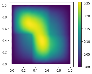
Let’s solve the thermal block problem and visualize the solution:
U = fom.solve([1.0, 0.1, 0.3, 0.1, 0.2, 1.0])
fom.visualize(U, title='Solution')
Each class in pyMOR that describes a Parameter-dependent mathematical
object, like the StationaryModel in our case, derives from
ParametricObject. ParametricObjects automatically determine the
Parameters they depend on from ParametricObjects that have been passed
as __init__ arguments and from the
parameters_own and
parameters_internal
attributes that have been set in __init__.
Let’s have a look:
print(fom.parameters)
{diffusion: 6}
This tells us, that the Parameters which
solve expects
should be a dictionary with one key 'diffusion' whose value is a one-dimensional
NumPy array of size 6, corresponding to the block structure of
the problem. However, as an exception to this rule, the interface methods of
Models allow simply passing the list [1.0, 0.1, 0.3, 0.1, 0.2, 1.0] by
internally calling parse.
Next we want to use the greedy algorithm
to reduce the problem. For this we need to choose a reductor which will keep
track of the reduced basis and perform the actual RB-projection. We will use
CoerciveRBReductor, which will
also assemble an error estimator to estimate the reduction error. This
will significantly speed up the basis generation, as we will only need to
solve the high-dimensional problem for those parameters in the training set
which are actually selected for basis extension. To control the condition of
the reduced system matrix, we must ensure that the generated basis is
orthonormal w.r.t. the H1_0-product on the solution space. For this we pass
the h1_0_semi_product attribute of the model as inner product to
the reductor, which will also use it for computing the Riesz representatives
required for error estimation. Moreover, we have to provide
the reductor with a ParameterFunctional which computes a lower bound for
the coercivity of the problem for given parameter values.
reductor = CoerciveRBReductor(
    fom,
    product=fom.h1_0_semi_product,
    coercivity_estimator=ExpressionParameterFunctional('min(diffusion)', fom.parameters)
)
Moreover, we need to select a training set of parameter values. The problem
p already comes with a ParameterSpace, from which we can easily sample
these values. E.g.:
training_set = p.parameter_space.sample_uniformly(4)
print(training_set[0])
{diffusion: [0.1, 0.1, 0.1, 0.1, 0.1, 0.1]}
Now we start the basis generation:
greedy_data = rb_greedy(fom, reductor, training_set, max_extensions=32)
The max_extensions parameter defines how many basis vectors we want to
obtain. greedy_data is a dictionary containing various data that has
been generated during the run of the algorithm:
print(greedy_data.keys())
dict_keys(['max_errs', 'max_err_mus', 'extensions', 'time', 'rom'])
The most important items is 'rom' which holds the reduced Model
obtained from applying our reductor with the final reduced basis.
rom = greedy_data['rom']
All vectors in pyMOR are stored in so called VectorArrays. For example
the solution U computed above is given as a VectorArray of length 1.
For the reduced basis we have:
RB = reductor.bases['RB']
print(type(RB))
print(len(RB))
print(RB.dim)
<class 'pymor.vectorarrays.numpy.NumpyVectorArray'>
32
5101
Let us check if the reduced basis really is orthonormal with respect to
the H1-product. For this we use the gramian
method:
import numpy as np
gram_matrix = RB.gramian(fom.h1_0_semi_product)
print(np.max(np.abs(gram_matrix - np.eye(32))))
1.478851763270228e-15
Looks good! We can now solve the reduced model for the same parameter values
as above. The result is a vector of coefficients w.r.t. the reduced basis, which is
currently stored in RB. To form the linear combination, we can use the
reconstruct method of the reductor:
u = rom.solve([1.0, 0.1, 0.3, 0.1, 0.2, 1.0])
print(u)
U_red = reductor.reconstruct(u)
print(U_red.dim)
[[ 0.56008169  0.19410562  0.00463453  0.01675562  0.04900982  0.07760119
  -0.08043888 -0.02889488 -0.03121126  0.26467367  0.13991773 -0.09805741
   0.16005484  0.04417512 -0.05245844 -0.00132281 -0.01304436  0.01330245
  -0.02185056  0.00625769 -0.00868736 -0.00115484  0.01895446 -0.00153234
   0.02306277  0.0035532   0.01061803 -0.00225572  0.00199581 -0.0068476
   0.00186538  0.0047302 ]]
5101
Finally we compute the reduction error and display the reduced solution along with the detailed solution and the error:
ERR = U - U_red
print(ERR.norm(fom.h1_0_semi_product))
fom.visualize((U, U_red, ERR),
              legend=('Detailed', 'Reduced', 'Error'),
              separate_colorbars=True)
[0.00480011]


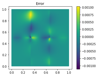
We can nicely observe that, as expected, the error is maximized along the jumps of the diffusion coefficient.
Download the code: getting_started.py getting_started.ipynb
Learning more
As a next step, you should read our Technical Overview which discusses the most important concepts and design decisions behind pyMOR. You can also follow our growing set of pyMOR Tutorials, which focus on specific aspects of pyMOR.
Should you have any problems regarding pyMOR, questions or feature requests, do not hesitate to contact us via GitHub discussions!