Run this tutorial
Click here to run this tutorial on binder:Tutorial: Model order reduction for port-Hamiltonian systems
In the first section, we introduce the class of port-Hamiltonian systems and their relationship to two other system-theoretic properties called passivity and positive realness. After introducing a toy example in the second section, we look into structure-preserving model reduction schemes for port-Hamiltonian systems in the third section.
Port-Hamiltonian LTI systems
Port-Hamiltonian systems have several favorable properties for modeling, control and simulation, for example, composability and stability. Furthermore, they adhere to a power balance equation. Port-Hamiltonian systems are especially suited for network-based modeling and problems involving multi-physics phenomena. We refer to [MU23] for a general introduction to port-Hamiltonian descriptor systems and their applications.
We say a LTI system is port-Hamiltonian if it can be expressed as
with \(H := Q^T E\), and if the structure matrix
and the dissipation matrix
satisfy \(H = H^T \succ 0\), \(\Gamma^T = -\Gamma\), and \(\mathcal{W} = \mathcal{W}^T \succcurlyeq 0\).
The quadratic (energy) function \(\mathcal{H}(x) := \tfrac{1}{2} x^T H x\), typically called Hamiltonian, corresponds to the energy stored in the system. In applications, \(E\) and/or \(Q\) often are identity matrices.
It is known that if the LTI system is minimal and stable, the following are equivalent:
The system is passive.
The system is port-Hamiltonian.
The system is positive real.
See for example [BU22] for more details.
In pyMOR, there exists a PHLTIModel class. Currently, pyMOR only supports
port-Hamiltonian systems with nonsingular E. PHLTIModel inherits from
LTIModel, so PHLTIModel can be used with all reductors that expect
an LTIModel. For model reduction, it is often desirable to preserve the
port-Hamiltonian structure, i.e., to compute a ROM that is also port-Hamiltonian.
If desired, a passive LTIModel can be converted into a PHLTIModel using
the from_passive_LTIModel method.
Consequentely, one option to preserve port-Hamiltonian structure is to use a reductor
that preserves passivity (but returns a ROM of type LTIModel) and convert the
ROM into a PHLTIModel in a post-processing step.
A toy problem: Mass-spring-damper chain
As a toy problem, we use a mass-spring-damper chain, which can be formulated as a port-Hamiltonian system (see [GPBvdS12]):

Here, the spring constants are denoted by \(k_i\) and the damping constants by
\(c_i\), \(i=1,\dots,n/2\).
The inputs \(u_1\) and \(u_2\) are the external forces on the first two
masses \(m_1\) and \(m_2\). The system outputs \(y_1\) and \(y_2\)
correspond to the velocities of the first two masses \(m_1\) and \(m_2\).
The toy problem is included in pyMOR in the pymor.models.examples module as
msd_example.
Structure-preserving model order reduction
pyMOR provides three reductors which can be used for model order reduction while preserving the port-Hamiltonian structure:
pH-IRKA (
PHIRKAReductor) [GPBvdS12],PRBT (
PRBTReductor) [DP84, GA04, HJS84],passivity preserving model reduction via spectral factorization (
SpectralFactorReductor) [BU22].
In this section, we apply all three reductors on our toy example and compare their performance. All three reductors are described in [BU22] in more detail.
Note: Currently, the PRBTReductor and
SpectralFactorReductor reductors require
the symmetric part of \(D\) (i.e., the \(S\) matrix in the port-Hamiltonian system)
to be nonsingular. The MSD example has a zero \(D\) matrix. Therefore,
we have to add a small regularization feedthrough term, i.e., we replace \(D\) with
\(D+\varepsilon I_m\). This is a limitation of the current implementation since the
numerical solution of the KYP-LMI is obtained by solving a related Riccati
equation, for instance
which is only possible if \(D + D^\top\) is nonsingular.
For from_passive_LTIModel, \(D + D^\top\) must be
nonsingular for the same reasons.
import numpy as np
from pymor.models.iosys import PHLTIModel
from pymor.models.examples import msd_example

J, R, G, P, S, N, E, Q = msd_example(50, 2)

# tolerance for solving the Riccati equation instead of KYP-LMI
# by introducing a regularization feedthrough term D
# (required for PRBTReductor and SpectralFactorReductor reductors)
S += np.eye(S.shape[0]) * 1e-12

fom = PHLTIModel.from_matrices(J, R, G, P=P, S=S, N=N, E=E, Q=Q, solver_options={'ricc_pos_lrcf': 'slycot'})
The ricc_pos_lrcf solver option refers to the solver used for the underlying
Riccati equation relevant for PRBTReductor and
SpectralFactorReductor. Possible choices are
scipy, slycot or pymess (if installed). Currently, we recommend slycot, since pyMOR’s
pymess binding does not support all use cases yet, and scipy gets into trouble if
the associated Hamiltonian pencil has eigenvalues close to the imaginary axis.
pH-IRKA
The pH-IRKA reductor PHIRKAReductor directly returns
a ROM of type PHLTIModel. pH-IRKA works similar to the standard IRKA reductor
IRKAReductor but with fewer degrees of freedom to preserve
the port-Hamiltonian structure. In more detail, the IRKA fixed-point iteration is performed,
but the left projection matrix is chosen as \(W = QV\), which then automatically yields a
reduced pH system with \(\hat{Q} = I_r\).
from pymor.reductors.ph.ph_irka import PHIRKAReductor

reductor = PHIRKAReductor(fom)
rom1 = reductor.reduce(10)
print(f'rom1 is of type {type(rom1).__qualname__}.')
rom1 is of type PHLTIModel.
Positive-real balanced truncation (PRBT)
Positive-real balanced truncation (PRBT) works analogously to the standard balanced truncation
method described in Tutorial: Reducing an LTI system using balanced truncation, but uses positive real controllability
and observability Gramians instead. PRBT preserves passivity but returns a ROM
of type LTIModel. Thus, we convert the ROM into a PHLTIModel in a
post-processing step. Note that PRBT can be used with any passive LTIModel FOM.
from pymor.reductors.bt import PRBTReductor

reductor = PRBTReductor(fom)
rom2 = reductor.reduce(10)
rom2 = rom2.with_(solver_options={'ricc_pos_lrcf': 'slycot'})
rom2 = PHLTIModel.from_passive_LTIModel(rom2)
print(f'rom2 is of type {type(rom2).__qualname__}.')
rom2 is of type PHLTIModel.
Passivity preserving model reduction via spectral factorization
The SpectralFactorReductor method
is a wrapper reductor for another generic reductor. The method extracts a
spectral factor from the FOM (this is only possible if the system is passive),
which subsequentely is reduced by a reductor specified by the user.
A spectral factor is a standard LTIModel, and hence any LTI reduction can be used.
For our example, we use the IRKAReductor as the inner reductor.
If the inner reductor returns a stable ROM, passivity is preserved.
The spectral factor method and PRBT are related since the computation of
the optimal spectral factor for model reduction depends on the computation of
the positive-real observability Gramian. The spectral factor method can be used with
any passive LTIModel FOM. Again, we convert the ROM of type LTIModel into a
PHLTIModel in a post-processing step.
from pymor.reductors.spectral_factor import SpectralFactorReductor
from pymor.reductors.h2 import IRKAReductor

reductor = SpectralFactorReductor(fom)
rom3 = reductor.reduce(
    lambda spectral_factor, mu : IRKAReductor(spectral_factor, mu).reduce(10)
)
rom3 = rom3.with_(solver_options={'ricc_pos_lrcf': 'slycot'})
rom3 = PHLTIModel.from_passive_LTIModel(rom3)
print(f'rom3 is of type {type(rom3).__qualname__}.')
rom3 is of type PHLTIModel.
Comparison
Let us compare the \(\mathcal{H}_2\) errors of the three methods:
err1 = fom - rom1
err2 = fom - rom2
err3 = fom - rom3

print(f'pHIRKA - Relative H2 error: {err1.h2_norm() / fom.h2_norm():.3e}')
print(f'PRBT - Relative H2 error: {err2.h2_norm() / fom.h2_norm():.3e}')
print(f'spectral_factor - Relative H2 error: {err3.h2_norm() / fom.h2_norm():.3e}')
pHIRKA - Relative H2 error: 2.430e-01
PRBT - Relative H2 error: 1.031e-02
spectral_factor - Relative H2 error: 3.240e-03
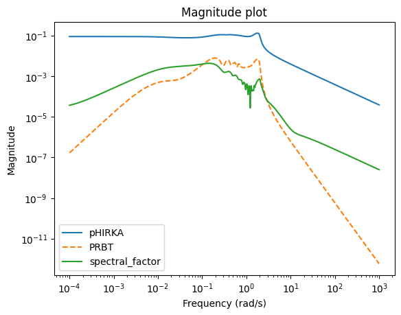
We can plot a magnitude plot of the three error systems:
import matplotlib.pyplot as plt
w = (1e-4, 1e3)
fig, ax = plt.subplots()
err1.transfer_function.mag_plot(w, ax=ax, label='pHIRKA')
err2.transfer_function.mag_plot(w, ax=ax, linestyle='--', label='PRBT')
err3.transfer_function.mag_plot(w, ax=ax, label='spectral_factor')
_ = ax.legend()
Download the code:
tutorial_ph.md,
tutorial_ph.ipynb.