Run this tutorial

Click here to run this tutorial on binder:
Please note that starting the notebook server may take a couple of minutes.

Getting Started

pyMOR includes a variety of model order reduction methods for different types of models. We illustrate how to use pyMOR on two basic examples and give pointers to further documentation.

Installation

pyMOR can be installed via pip. To follow this guide, pyMOR should be installed with GUI support:

pip install pymor[gui]

If you follow along in a Jupyter notebook, you should install pyMOR using the jupyter extra:

pip install pymor[jupyter]

We also provide conda-forge packages. For further details see README.md.

Reduced Basis Method for Elliptic Problem

Here we show how to reduce a parametric linear elliptic problem using the Reduced Basis (RB) method. As an example we use a standard 2x2 thermal-block problem, which is given by the elliptic equation

\[ -\nabla \cdot [d(x, \mu) \nabla u(x, \mu)] = 1 \]

on the domain \([0, 1]^2\) with Dirichlet zero boundary values. The domain is partitioned into 2x2 blocks and the diffusion function \(d(x, \mu)\) is constant on each such block \(i\) with value \(\mu_i\).

(0,1)---------(1,1)
|        |        |
|  μ_2   |  μ_3   |
|        |        |
|------------------
|        |        |
|  μ_0   |  μ_1   |
|        |        |
(0,0)---------(1,0)

After discretization, the model has the form

\[ (L + \mu_0 L_0 + \mu_1 L_1 + \mu_2 L_2 + \mu_3 L_3) u(\mu) = f \]

We can obtain this discrete full-order model in pyMOR using the thermal_block_example function from the pymor.models.examples module:

from pymor.models.examples import thermal_block_example

fom_tb = thermal_block_example()

This uses pyMOR’s builtin discretization toolkit to construct the model. In the builtin-discretizer tutorial you learn how to define your own models using this toolkit.

fom_tb is an instance of StationaryModel, which encodes the mathematical structure of the model through its Operators:

fom_tb

StationaryModel(
    LincombOperator(
        (NumpyMatrixOperator(<20201x20201 sparse, 400 nnz>, source_id='STATE', range_id='STATE', name='boundary_part'),
         NumpyMatrixOperator(<20201x20201 sparse, 24801 nnz>, source_id='STATE', range_id='STATE', name='diffusion_0'),
         NumpyMatrixOperator(<20201x20201 sparse, 24801 nnz>, source_id='STATE', range_id='STATE', name='diffusion_1'),
         NumpyMatrixOperator(<20201x20201 sparse, 24801 nnz>, source_id='STATE', range_id='STATE', name='diffusion_2'),
         NumpyMatrixOperator(<20201x20201 sparse, 24801 nnz>, source_id='STATE', range_id='STATE', name='diffusion_3')),
        (1.0,
         ProjectionParameterFunctional('diffusion', size=4, index=0, name='diffusion_0_0'),
         ProjectionParameterFunctional('diffusion', size=4, index=1, name='diffusion_1_0'),
         ProjectionParameterFunctional('diffusion', size=4, index=2, name='diffusion_0_1'),
         ProjectionParameterFunctional('diffusion', size=4, index=3, name='diffusion_1_1')),
        name='ellipticOperator'),
    NumpyMatrixOperator(<20201x1 dense>, range_id='STATE'),
    output_functional=ZeroOperator(NumpyVectorSpace(0), NumpyVectorSpace(20201, id='STATE')),
    products={h1: NumpyMatrixOperator(<20201x20201 sparse, 140601 nnz>, source_id='STATE', range_id='STATE'),
              h1_semi: NumpyMatrixOperator(<20201x20201 sparse, 100201 nnz>, source_id='STATE', range_id='STATE', name='h1_semi'),
              l2: NumpyMatrixOperator(<20201x20201 sparse, 140601 nnz>, source_id='STATE', range_id='STATE', name='l2'),
              h1_0: NumpyMatrixOperator(<20201x20201 sparse, 137417 nnz>, source_id='STATE', range_id='STATE'),
              h1_0_semi: NumpyMatrixOperator(<20201x20201 sparse, 98609 nnz>, source_id='STATE', range_id='STATE', name='h1_0_semi'),
              l2_0: NumpyMatrixOperator(<20201x20201 sparse, 137417 nnz>, source_id='STATE', range_id='STATE', name='l2_0')},
    visualizer=PatchVisualizer(
                   TriaGrid(num_intervals=(100, 100), domain=array([[0, 0], [1, 1]])),
                   bounding_box=array([[0, 0], [1, 1]]),
                   backend='jupyter'),
    name='ThermalBlock((2, 2))_CG')

Its parameters can also be accessed:

fom_tb.parameters

Parameters({diffusion: 4})

Let us show the solution for particular parameter values:

mu = [0.1, 0.2, 0.5, 1]
U = fom_tb.solve(mu)
fom_tb.visualize(U)

To construct a reduced-order model using the reduced basis method, we first need to create a reductor which projects the model onto a given reduced space:

from pymor.parameters.functionals import ExpressionParameterFunctional
from pymor.reductors.coercive import CoerciveRBReductor

reductor = CoerciveRBReductor(
    fom_tb,
    product=fom_tb.h1_0_semi_product,
    coercivity_estimator=ExpressionParameterFunctional('min(diffusion)',
                                                       fom_tb.parameters)
)

We use here CoerciveRBReductor, which also assembles an a posterior error estimator for the error w.r.t. the \(H^1_0\)-seminorm. For that estimator, an parameter-dependent lower bound for the coercivity constant of the problem is provided as an ExpressionParameterFunctional.

Using this reductor and its error estimator, we can build a reduced space with corresponding reduced-order model using a weak greedy algorithm:

from pymor.algorithms.greedy import rb_greedy

parameter_space = fom_tb.parameters.space(0.1, 1)
greedy_data = rb_greedy(fom_tb, reductor, parameter_space.sample_randomly(1000),
                        rtol=1e-2)
rom_tb = greedy_data['rom']

Here, the greedy algorithm operates on a randomly chosen set of 1000 training parameters from the ParameterSpace of admissible parameter values returned by thermal_block_example.

We can see that the reduced-order model is also a StationaryModel, but of lower order:

rom_tb

StationaryModel(
    LincombOperator(
        (NumpyMatrixOperator(<12x12 dense>),
         NumpyMatrixOperator(<12x12 dense>),
         NumpyMatrixOperator(<12x12 dense>),
         NumpyMatrixOperator(<12x12 dense>),
         NumpyMatrixOperator(<12x12 dense>)),
        (1.0,
         ProjectionParameterFunctional('diffusion', size=4, index=0, name='diffusion_0_0'),
         ProjectionParameterFunctional('diffusion', size=4, index=1, name='diffusion_1_0'),
         ProjectionParameterFunctional('diffusion', size=4, index=2, name='diffusion_0_1'),
         ProjectionParameterFunctional('diffusion', size=4, index=3, name='diffusion_1_1'))),
    NumpyMatrixOperator(<12x1 dense>),
    output_functional=ZeroOperator(NumpyVectorSpace(0), NumpyVectorSpace(12)),
    products={h1: NumpyMatrixOperator(<12x12 dense>),
              h1_semi: NumpyMatrixOperator(<12x12 dense>),
              l2: NumpyMatrixOperator(<12x12 dense>),
              h1_0: NumpyMatrixOperator(<12x12 dense>),
              h1_0_semi: NumpyMatrixOperator(<12x12 dense>),
              l2_0: NumpyMatrixOperator(<12x12 dense>)},
    error_estimator=CoerciveRBEstimator(
                        ResidualOperator(
                            LincombOperator(
                                (NumpyMatrixOperator(<47x12 dense>),
                                 NumpyMatrixOperator(<47x12 dense>),
                                 NumpyMatrixOperator(<47x12 dense>),
                                 NumpyMatrixOperator(<47x12 dense>),
                                 NumpyMatrixOperator(<47x12 dense>)),
                                (1.0,
                                 ProjectionParameterFunctional('diffusion', size=4, index=0, name='diffusion_0_0'),
                                 ProjectionParameterFunctional('diffusion', size=4, index=1, name='diffusion_1_0'),
                                 ProjectionParameterFunctional('diffusion', size=4, index=2, name='diffusion_0_1'),
                                 ProjectionParameterFunctional('diffusion', size=4, index=3, name='diffusion_1_1'))),
                            NumpyMatrixOperator(<47x1 dense>)),
                        (1, 4, 8, 12, 16, 20, 24, 27, 31, 35, 39, 43, 47),
                        ExpressionParameterFunctional('min(diffusion)', {diffusion: 4}),
                        projected_output_adjoint=ZeroOperator(NumpyVectorSpace(0), NumpyVectorSpace(0))),
    name='ThermalBlock((2, 2))_CG_reduced')

We can compute the reduced-order model’s reconstructed solution for the same parameter value and show the error:

Urom = rom_tb.solve(mu)
Urec = reductor.reconstruct(Urom)
fom_tb.visualize(U - Urec)

Finally, we check that the reduced-order model is indeed faster:

from time import perf_counter
tic = perf_counter()
fom_tb.solve(mu)
toc = perf_counter()
rom_tb.solve(mu)
tac = perf_counter()
print(f't_fom: {toc-tic}  t_rom: {tac-toc}  speedup: {(toc-tic)/(tac-toc)}')

t_fom: 0.0849742959999844  t_rom: 0.0006372999999939566  speedup: 133.3348438738274

Balanced Truncation for LTI System

Here we consider a synthetic linear time-invariant (LTI) system of the form

\[\begin{split} \begin{align*} \dot{x}(t) & = A x(t) + B u(t), \\ y(t) & = C x(t), \end{align*} \end{split}\]

where \(x\) is the state, \(u\) is the input, and \(y\) is the output.

from pymor.models.examples import penzl_example

fom_lti = penzl_example()

The result is an LTIModel:

fom_lti

LTIModel(
    NumpyMatrixOperator(<1006x1006 sparse, 1012 nnz>, source_id='STATE', range_id='STATE'),
    NumpyMatrixOperator(<1006x1 dense>, range_id='STATE'),
    NumpyMatrixOperator(<1x1006 dense>, source_id='STATE'),
    D=ZeroOperator(NumpyVectorSpace(1), NumpyVectorSpace(1)),
    E=IdentityOperator(NumpyVectorSpace(1006, id='STATE')),
    presets={})

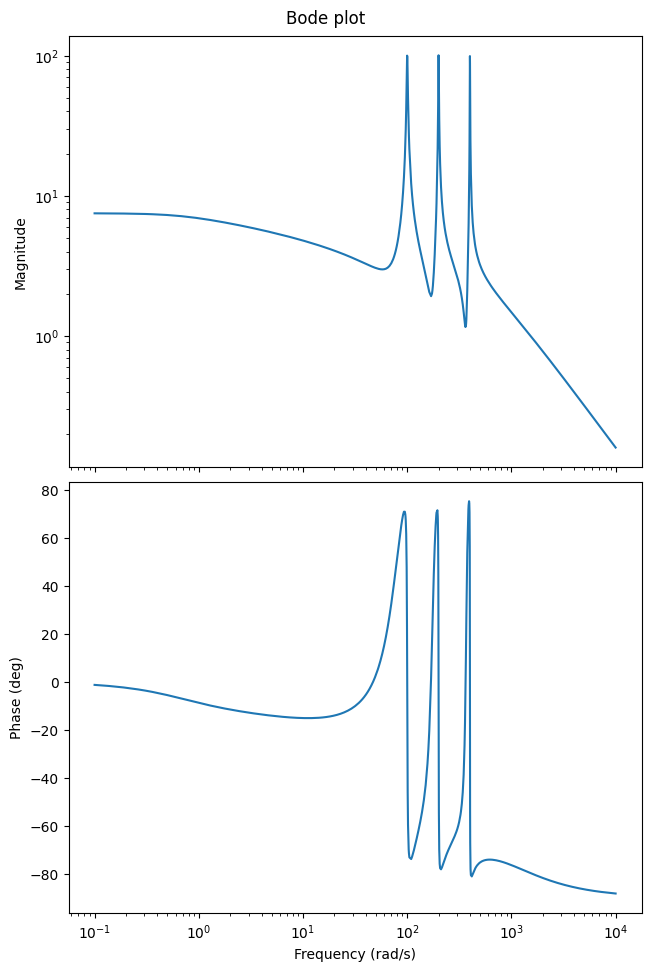
We can use the Bode plot to show the frequency response of the LTI system, i.e., to see which input frequencies are amplified and phase-shifted in the output:

w = (1e-1, 1e4)
_ = fom_lti.transfer_function.bode_plot(w)

Note that if you do not run this code in a Jupyter notebook, you probably need to manually show the plot:

from matplotlib import pyplot as plt
plt.show()

We can run balanced truncation to obtain a reduced-order model.

from pymor.reductors.bt import BTReductor

bt = BTReductor(fom_lti)
rom_lti = bt.reduce(10)

The reduced-order model is again an LTIModel, but of lower order.

rom_lti

LTIModel(
    NumpyMatrixOperator(<10x10 dense>),
    NumpyMatrixOperator(<10x1 dense>),
    NumpyMatrixOperator(<1x10 dense>),
    D=ZeroOperator(NumpyVectorSpace(1), NumpyVectorSpace(1)),
    E=NumpyMatrixOperator(<10x10 dense>),
    presets={},
    name='LTIModel_reduced')

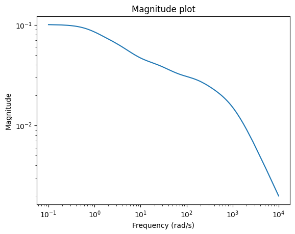
Looking at the error system, we can see which frequencies are well approximated.

err_lti = fom_lti - rom_lti
_ = err_lti.transfer_function.mag_plot(w)

Running Demo Scripts

pyMOR ships several example scripts that showcase various features of the library. While many features are also covered in our pyMOR Tutorials, the demos are more extensive and often have various command-line flags which allow to run the script for different parameters or problems. All demos can be found in the src/pymordemos directory of the source repository.

The demo scripts can be launched directly from the source tree:

./thermalblock.py --plot-err --plot-solutions 3 2 3 32

or by using the pymor-demo script that is installed with pyMOR:

pymor-demo thermalblock --plot-err --plot-solutions 3 2 3 32

Learning More

You can find more details on the above approaches, and even more, in the pyMOR Tutorials. Specific questions are answered in GitHub discussions. The Technical Overview provides discussion on fundamental pyMOR concepts and design decisions.

Should you have any problems regarding pyMOR, questions or feature requests, do not hesitate to contact us via GitHub discussions or email!

Download the code: getting_started.md getting_started.ipynb