Tutorial: Reducing a heat equation using balanced truncation
Heat equation
We consider the following one-dimensional heat equation over \((0, 1)\) with two inputs \(u_1, u_2\) and three outputs \(y_1, y_2, y_2\):
In the following, we will create a discretized Model and reduce it using the
balanced truncation method to approximate the mapping from inputs
\(u = (u_1, u_2)\) to outputs \(y = (y_1, y_2, y_3)\).
Discretized model
We need to construct a linear time-invariant (LTI) system
In pyMOR, these models are captured by LTIModels from the
pymor.models.iosys module.
There are many ways of building an LTIModel.
Here, we show how to build one from custom matrices instead of using a
discretizer as in Tutorial: Using pyMOR’s discretization toolkit and the
to_lti of InstationaryModel.
In particular, we will use the
from_matrices method of LTIModel, which
instantiates an LTIModel from NumPy or SciPy matrices.
First, we do the necessary imports.
import matplotlib.pyplot as plt
import numpy as np
import scipy.sparse as sps
from pymor.models.iosys import LTIModel
from pymor.reductors.bt import BTReductor
Next, we can assemble the matrices based on a centered finite difference approximation:
k = 50
n = 2 * k + 1

A = sps.diags(
    [(n - 1) * [(n - 1)**2], n * [-2 * (n - 1)**2], (n - 1) * [(n - 1)**2]],
    [-1, 0, 1],
    format='lil',
)
A[0, 0] = A[-1, -1] = -2 * n * (n - 1)
A[0, 1] = A[-1, -2] = 2 * (n - 1)**2
A = A.tocsc()

B = np.zeros((n, 2))
B[:, 0] = 1
B[0, 1] = 2 * (n - 1)

C = np.zeros((3, n))
C[0, 0] = C[1, k] = C[2, -1] = 1
Then, we can create an LTIModel:
fom = LTIModel.from_matrices(A, B, C)
We can get the internal representation of the LTIModel fom
fom
LTIModel(
    NumpyMatrixOperator(<101x101 sparse, 301 nnz>, source_id='STATE', range_id='STATE'),
    NumpyMatrixOperator(<101x2 dense>, range_id='STATE'),
    NumpyMatrixOperator(<3x101 dense>, source_id='STATE'),
    D=ZeroOperator(NumpyVectorSpace(3), NumpyVectorSpace(2)),
    E=IdentityOperator(NumpyVectorSpace(101, id='STATE')))
From this, we see that the matrices were wrapped in NumpyMatrixOperators,
while default values were chosen for \(D\) and \(E\) matrices
(respectively, zero and identity). The operators in an LTIModel can be
accessed directly, e.g., fom.A.
We can also see some basic information from fom’s string representation
print(fom)
LTIModel
    class: LTIModel
    number of equations: 101
    number of inputs:    2
    number of outputs:   3
    continuous-time
    linear time-invariant
    solution_space:  NumpyVectorSpace(101, id='STATE')
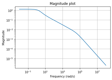
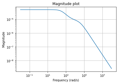
To visualize the behavior of the fom, we can draw its magnitude plot, i.e.,
a visualization of the mapping \(\omega \mapsto H(i \omega)\), where
\(H(s) = C (s E - A)^{-1} B + D\) is the transfer function of the system.
w = np.logspace(-2, 8, 50)
fom.mag_plot(w)
plt.grid()
Plotting the Hankel singular values shows us how well an LTI system can be approximated by a reduced-order model
hsv = fom.hsv()
fig, ax = plt.subplots()
ax.semilogy(range(1, len(hsv) + 1), hsv, '.-')
ax.set_title('Hankel singular values')
ax.grid()
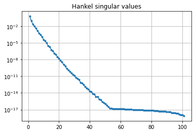
As expected for a heat equation, the Hankel singular values decay rapidly.
Running balanced truncation
The balanced truncation method consists of finding a balanced realization of the full-order LTI system and truncating it to obtain a reduced-order model. In particular, there exist invertible transformation matrices \(T, S \in \mathbb{R}^{n \times n}\) such that the equivalent full-order model with \(\widetilde{E} = S^T E T = I\), \(\widetilde{A} = S^T A T\), \(\widetilde{B} = S^T B\), \(\widetilde{C} = C T\) has Gramians \(\widetilde{P}\) and \(\widetilde{Q}\), i.e., solutions to Lyapunov equations
such that \(\widetilde{P} = \widetilde{Q} = \Sigma = \operatorname{diag}(\sigma_i)\), where \(\sigma_i\) are the Hankel singular values. Then, taking as basis matrices \(V, W \in \mathbb{R}^{n \times r}\) the first \(r\) columns of \(T\) and \(S\) (possibly after orthonormalization), gives a reduced-order model
with \(\widehat{E} = W^T E V\), \(\widehat{A} = W^T A V\), \(\widehat{B} = W^T B\), \(\widehat{C} = C V\), which satisfies the \(\mathcal{H}_\infty\) (i.e., induced \(\mathcal{L}_2\)) error bound
Note that any reduced-order model (not only from balanced truncation) satisfies the lower bound
To run balanced truncation in pyMOR, we first need the reductor object
bt = BTReductor(fom)
Calling its reduce method runs the
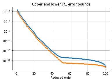
balanced truncation algorithm. This reductor additionally has an error_bounds
method which can compute the a priori \(\mathcal{H}_\infty\) error bounds
based on the Hankel singular values:
error_bounds = bt.error_bounds()
fig, ax = plt.subplots()
ax.semilogy(range(1, len(error_bounds) + 1), error_bounds, '.-')
ax.semilogy(range(1, len(hsv)), hsv[1:], '.-')
ax.set_xlabel('Reduced order')
ax.set_title(r'Upper and lower $\mathcal{H}_\infty$ error bounds')
ax.grid()
To get a reduced-order model of order 10, we call the reduce method with the
appropriate argument:
rom = bt.reduce(10)
Instead, or in addition, a tolerance for the \(\mathcal{H}_\infty\) error
can be specified, as well as the projection algorithm (by default, the
balancing-free square root method is used).
The used Petrov-Galerkin bases are stored in bt.V and bt.W.
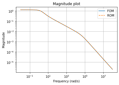
We can compare the magnitude plots between the full-order and reduced-order models
fig, ax = plt.subplots()
fom.mag_plot(w, ax=ax, label='FOM')
rom.mag_plot(w, ax=ax, linestyle='--', label='ROM')
ax.legend()
ax.grid()
and plot the magnitude plot of the error system
(fom - rom).mag_plot(w)
plt.grid()
We can compute the relative errors in \(\mathcal{H}_\infty\) or \(\mathcal{H}_2\) (or Hankel) norm
print(f'Relative Hinf error: {(fom - rom).hinf_norm() / fom.hinf_norm():.3e}')
print(f'Relative H2 error:   {(fom - rom).h2_norm() / fom.h2_norm():.3e}')
Relative Hinf error: 3.702e-05
Relative H2 error:   6.399e-04
Note
To compute the \(\mathcal{H}_\infty\) norms, pyMOR uses the dense solver from Slycot, and therefore all of the operators have to be converted to dense matrices. For large systems, this may be very expensive.
Download the code: tutorial_bt.py tutorial_bt.ipynb