Run this tutorial

Click here to run this tutorial on mybinder.org:
Please note that starting the notebook server may take a couple of minutes.

Tutorial: Model order reduction with artificial neural networks

Recent success of artificial neural networks led to the development of several methods for model order reduction using neural networks. pyMOR provides the functionality for a simple approach developed by Hesthaven and Ubbiali in [HU18]. For training and evaluation of the neural networks, PyTorch is used.

In this tutorial we will learn about feedforward neural networks, the basic idea of the approach by Hesthaven et al., and how to use it in pyMOR.

Feedforward neural networks

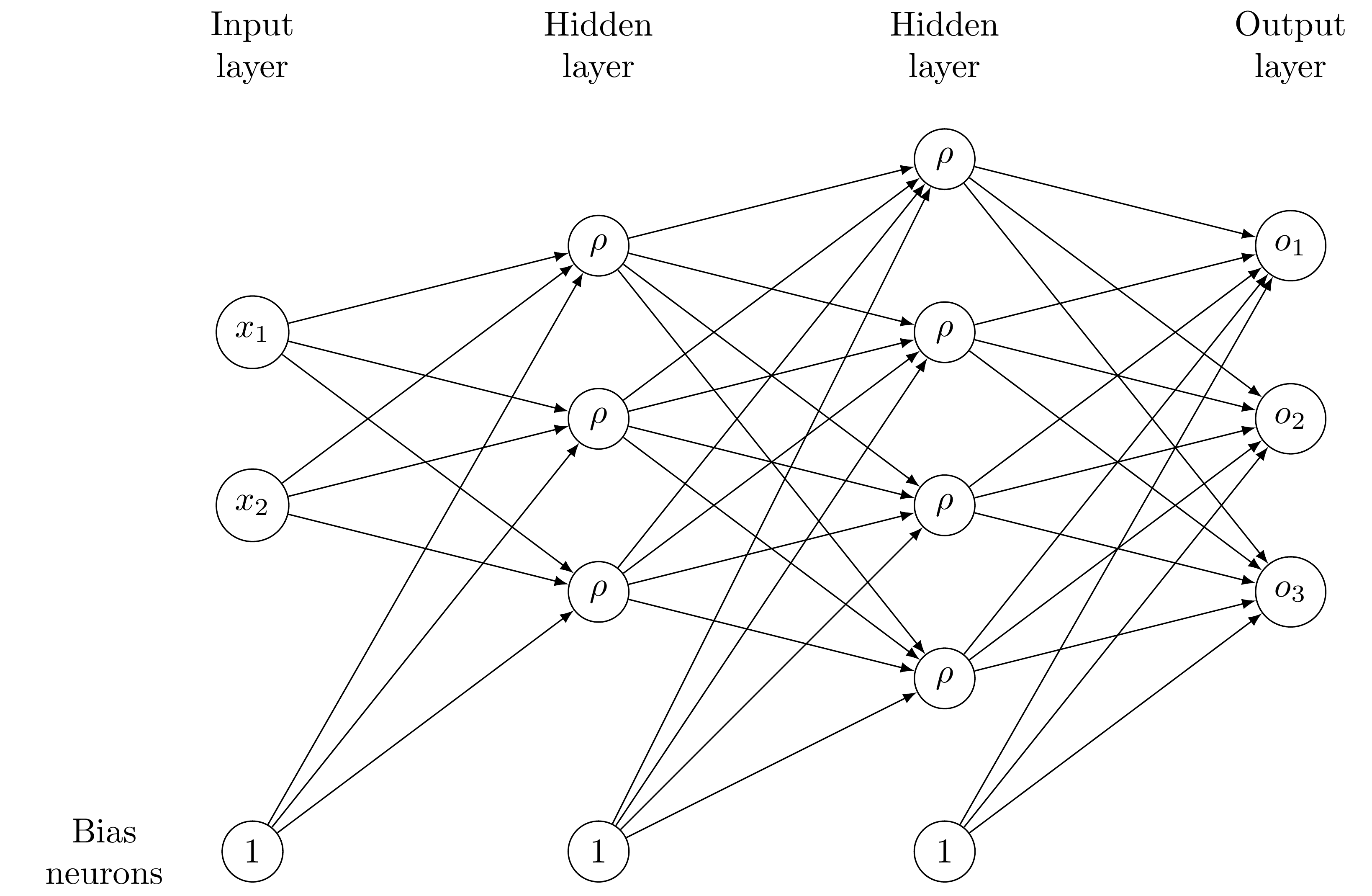
We aim at approximating a mapping \(h\colon\mathcal{P}\rightarrow Y\) between some input space \(\mathcal{P}\subset\mathbb{R}^p\) (in our case the parameter space) and an output space \(Y\subset\mathbb{R}^m\) (in our case the reduced space), given a set \(S=\{(\mu_i,h(\mu_i))\in\mathcal{P}\times Y: i=1,\dots,N\}\) of samples, by means of an artificial neural network. In this context, neural networks serve as a special class of functions that are able to “learn” the underlying structure of the sample set \(S\) by adjusting their weights. More precisely, feedforward neural networks consist of several layers, each comprising a set of neurons that are connected to neurons in adjacent layers. A so-called “weight” is assigned to each of those connections. The weights in the neural network can be adjusted while fitting the neural network to the given sample set. For a given input \(\mu\in\mathcal{P}\), the weights between the input layer and the first hidden layer (the one after the input layer) are multiplied with the respective values in \(\mu\) and summed up. Subsequently, a so-called “bias” (also adjustable during training) is added and the result is assigned to the corresponding neuron in the first hidden layer. Before passing those values to the following layer, a (non-linear) activation function \(\rho\colon\mathbb{R}\rightarrow\mathbb{R}\) is applied. If \(\rho\) is linear, the function implemented by the neural network is affine, since solely affine operations were performed. Hence, one usually chooses a non-linear activation function to introduce non-linearity in the neural network and thus increase its approximation capability. In some sense, the input \(\mu\) is passed through the neural network, affine-linearly combined with the other inputs and non-linearly transformed. These steps are repeated in several layers.

The following figure shows a simple example of a neural network with two hidden layers, an input size of two and an output size of three. Each edge between neurons has a corresponding weight that is learnable in the training phase.

To train the neural network, one considers a so-called “loss function”, that measures how the neural network performs on the training set \(S\), i.e. how accurately the neural network reproduces the output \(h(\mu_i)\) given the input \(\mu_i\). The weights of the neural network are adjusted iteratively such that the loss function is successively minimized. To this end, one typically uses a Quasi-Newton method for small neural networks or a (stochastic) gradient descent method for deep neural networks (those with many hidden layers).

A possibility to use feedforward neural networks in combination with reduced basis methods will be introduced in the following section.

A non-intrusive reduced order method using artificial neural networks

We now assume that we are given a parametric pyMOR Model for which we want to compute a reduced order surrogate Model using a neural network. In this example, we consider the following two-dimensional diffusion problem with parametrized diffusion, right hand side and Dirichlet boundary condition:

\[-\nabla \cdot \big(\sigma(x, \mu) \nabla u(x, \mu) \big) = f(x, \mu),\quad x=(x_1,x_2) \in \Omega,\]

on the domain \(\Omega:= (0, 1)^2 \subset \mathbb{R}^2\) with data functions \(f((x_1, x_2), \mu) = 10 \cdot \mu + 0.1\), \(\sigma((x_1, x_2), \mu) = (1 - x_1) \cdot \mu + x_1\), where \(\mu \in (0.1, 1)\) denotes the parameter. Further, we apply the Dirichlet boundary conditions

\[u((x_1, x_2), \mu) = 2x_1\mu + 0.5,\quad x=(x_1, x_2) \in \partial\Omega.\]

We discretize the problem using pyMOR’s builtin discretization toolkit as explained in Tutorial: Using pyMOR’s discretization toolkit:

from pymor.basic import *

problem = StationaryProblem(
      domain=RectDomain(),

      rhs=LincombFunction(
          [ExpressionFunction('10', 2), ConstantFunction(1., 2)],
          [ProjectionParameterFunctional('mu'), 0.1]),

      diffusion=LincombFunction(
          [ExpressionFunction('1 - x[0]', 2), ExpressionFunction('x[0]', 2)],
          [ProjectionParameterFunctional('mu'), 1]),

      dirichlet_data=LincombFunction(
          [ExpressionFunction('2 * x[0]', 2), ConstantFunction(1., 2)],
          [ProjectionParameterFunctional('mu'), 0.5]),

      name='2DProblem'
  )

fom, _ = discretize_stationary_cg(problem, diameter=1/50)

Since we employ a single Parameter, and thus use the same range for each parameter, we can create the ParameterSpace using the following line:

parameter_space = fom.parameters.space((0.1, 1))

The main idea of the approach by Hesthaven et al. is to approximate the mapping from the Parameters to the coefficients of the respective solution in a reduced basis by means of a neural network. Thus, in the online phase, one performs a forward pass of the Parameters through the neural networks and obtains the approximated reduced coordinates. To derive the corresponding high-fidelity solution, one can further use the reduced basis and compute the linear combination defined by the reduced coefficients. The reduced basis is created via POD.

The method described above is “non-intrusive”, which means that no deep insight into the model or its implementation is required and it is completely sufficient to be able to generate full order snapshots for a randomly chosen set of parameters. This is one of the main advantages of the proposed approach, since one can simply train a neural network, check its performance and resort to a different method if the neural network does not provide proper approximation results.

In pyMOR, there exists a training routine for feedforward neural networks. This procedure is part of a reductor and it is not necessary to write a custom training algorithm for each specific problem. However, it is sometimes necessary to try different architectures for the neural network to find the one that best fits the problem at hand. In the reductor, one can easily adjust the number of layers and the number of neurons in each hidden layer, for instance. Furthermore, it is also possible to change the deployed activation function.

To train the neural network, we create a training and a validation set consisting of 100 and 20 randomly chosen parameter values, respectively:

training_set = parameter_space.sample_uniformly(100)
validation_set = parameter_space.sample_randomly(20)

In this tutorial, we construct the reduced basis such that no more modes than required to bound the l2-approximation error by a given value are used. The l2-approximation error is the error of the orthogonal projection (in the l2-sense) of the training snapshots onto the reduced basis. That is, we prescribe l2_err in the reductor. It is also possible to determine a relative or absolute tolerance (in the singular values) that should not be exceeded on the training set. Further, one can preset the size of the reduced basis.

The training is aborted when a neural network that guarantees our prescribed tolerance is found. If we set ann_mse to None, this function will automatically train several neural networks with different initial weights and select the one leading to the best results on the validation set. We can also set ann_mse to 'like_basis'. Then, the algorithm tries to train a neural network that leads to a mean squared error on the training set that is as small as the error of the reduced basis. If the maximal number of restarts is reached without finding a network that fulfills the tolerances, an exception is raised. In such a case, one could try to change the architecture of the neural network or switch to ann_mse=None which is guaranteed to produce a reduced order model (perhaps with insufficient approximation properties).

We can now construct a reductor with prescribed error for the basis and mean squared error of the neural network:

from pymor.reductors.neural_network import NeuralNetworkReductor

reductor = NeuralNetworkReductor(fom,
                                 training_set,
                                 validation_set,
                                 l2_err=1e-5,
                                 ann_mse=1e-5)

To reduce the model, i.e. compute a reduced basis via POD and train the neural network, we use the respective function of the NeuralNetworkReductor:

rom = reductor.reduce(restarts=100)

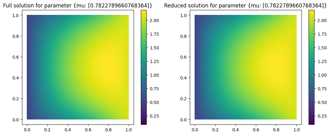
We are now ready to test our reduced model by solving for a random parameter value the full problem and the reduced model and visualize the result:

mu = parameter_space.sample_randomly()

U = fom.solve(mu)
U_red = rom.solve(mu)
U_red_recon = reductor.reconstruct(U_red)

fom.visualize((U, U_red_recon),
              legend=(f'Full solution for parameter {mu}', f'Reduced solution for parameter {mu}'))

Finally, we measure the error of our neural network and the performance compared to the solution of the full order problem on a training set. To this end, we sample randomly some parameter values from our ParameterSpace:

test_set = parameter_space.sample_randomly(10)

Next, we create empty solution arrays for the full and reduced solutions and an empty list for the speedups:

U = fom.solution_space.empty(reserve=len(test_set))
U_red = fom.solution_space.empty(reserve=len(test_set))

speedups = []

Now, we iterate over the test set, compute full and reduced solutions to the respective parameters and measure the speedup:

import time

for mu in test_set:
    tic = time.perf_counter()
    U.append(fom.solve(mu))
    time_fom = time.perf_counter() - tic

    tic = time.perf_counter()
    U_red.append(reductor.reconstruct(rom.solve(mu)))
    time_red = time.perf_counter() - tic

    speedups.append(time_fom / time_red)

We can now derive the absolute and relative errors on the training set as

absolute_errors = (U - U_red).norm()
relative_errors = (U - U_red).norm() / U.norm()

The average absolute error amounts to

import numpy as np

np.average(absolute_errors)

0.004755120599120671

On the other hand, the average relative error is

np.average(relative_errors)

5.2114466909876e-05

Using neural networks results in the following median speedup compared to solving the full order problem:

np.median(speedups)

15.845718265069577

Since NeuralNetworkReductor only calls the solve method of the Model, it can easily be applied to Models originating from external solvers, without requiring any access to Operators internal to the solver.

Direct approximation of output quantities

Thus far, we were mainly interested in approximating the solution state \(u(\mu)\equiv u(\cdot,\mu)\) for some parameter \(\mu\). If we consider an output functional \(\mathcal{J}(\mu):= J(u(\mu), \mu)\), one can use the reduced solution \(u_N(\mu)\) for computing the output as \(\mathcal{J}(\mu)\approx J(u_N(\mu),\mu)\). However, when dealing with neural networks, one could also think about directly learning the mapping from parameter to output. That is, one can use a neural network to approximate \(\mathcal{J}\colon\mathcal{P}\to\mathbb{R}^q\), where \(q\in\mathbb{N}\) denotes the output dimension.

In the following, we will extend our problem from the last section by an output functional and use the NeuralNetworkStatefreeOutputReductor to derive a reduced model that can solely be used to solve for the output quantity without computing a reduced state at all.

For the definition of the output, we define the output of out problem as the l2-product of the solution with the right hand side respectively Dirichlet boundary data of our original problem:

problem = problem.with_(outputs=[('l2', problem.rhs), ('l2_boundary', problem.dirichlet_data)])

Consequently, the output dimension is \(q=2\). After adjusting the problem definition, we also have to update the full order model to be aware of the output quantities:

fom, _ = discretize_stationary_cg(problem, diameter=1/50)

We can now import the NeuralNetworkStatefreeOutputReductor and initialize the reductor using the same data as before:

from pymor.reductors.neural_network import NeuralNetworkStatefreeOutputReductor

output_reductor = NeuralNetworkStatefreeOutputReductor(fom,
                                                       training_set,
                                                       validation_set,
                                                       validation_loss=1e-5)

Similar to the NeuralNetworkReductor, we can call reduce to obtain a reduced order model. In this case, reduce trains a neural network to approximate the mapping from parameter to output directly. Therefore, we can only use the resulting reductor to solve for the outputs and not for state approximations. The NeuralNetworkReductor though can be used to do both by calling solve respectively output (if we had initialized the NeuralNetworkReductor with the problem including the output quantities).

We now perform the reduction and run some tests with the resulting NeuralNetworkStatefreeOutputModel:

output_rom = output_reductor.reduce(restarts=100)

outputs = []
outputs_red = []
outputs_speedups = []

for mu in test_set:
    tic = time.perf_counter()
    outputs.append(fom.output(mu=mu))
    time_fom = time.perf_counter() - tic

    tic = time.perf_counter()
    outputs_red.append(output_rom.output(mu=mu))
    time_red = time.perf_counter() - tic

    outputs_speedups.append(time_fom / time_red)

outputs = np.squeeze(np.array(outputs))
outputs_red = np.squeeze(np.array(outputs_red))

outputs_absolute_errors = np.abs(outputs - outputs_red)
outputs_relative_errors = np.abs(outputs - outputs_red) / np.abs(outputs)

The average absolute error (component-wise) on the training set is given by

np.average(outputs_absolute_errors)

0.001393936984678279

The average relative error is

np.average(outputs_relative_errors)

0.00041834554676528087

and the median of the speedups amounts to

np.median(outputs_speedups)

14.31403360041245

Neural networks for instationary problems

To solve instationary problems using neural networks, we have extended the NeuralNetworkReductor to the NeuralNetworkInstationaryReductor, which treats time as an additional parameter (see [WHR19]). The resulting NeuralNetworkInstationaryModel passes the input, together with the current time instance, through the neural network in each time step to obtain reduced coefficients. In the same fashion, there exists a NeuralNetworkInstationaryStatefreeOutputReductor and the corresponding NeuralNetworkInstationaryStatefreeOutputModel.

A slightly different approach that is also implemented in pyMOR and uses a different type of neural network is described in the following section.

Long short-term memory neural networks for instationary problems

So-called recurrent neural networks are especially well-suited for capturing time-dependent dynamics. These types of neural networks can treat input sequences of variable length (in our case sequences with a variable number of time steps) and store internal states that are passed from one time step to the next. Therefore, these networks implement an internal memory that keeps information over time. Furthermore, for each element of the input sequence, the same neural network is applied.

In the NeuralNetworkLSTMInstationaryModel and the corresponding NeuralNetworkLSTMInstationaryReductor, we make use of a specific type of recurrent neural network, namely a so-called long short-term memory neural network (LSTM), first introduced in [HS97], that tries to avoid problems like vanishing or exploding gradients that often occur during training of recurrent neural networks.

The architecture of an LSTM neural network

In an LSTM neural network, multiple so-called LSTM cells are chained with each other such that the cell state \(c_k\) and the hidden state \(h_k\) of the \(k\)-th LSTM cell serve as the input hidden states for the \(k+1\)-th LSTM cell. Therefore, information from former time steps can be available later. Each LSTM cell takes an input \(\mu(t_k)\) and produces an output \(o(t_k)\). The following figure shows the general structure of an LSTM neural network that is also implemented in the same way in pyMOR:

The LSTM cell

The main building block of an LSTM network is the LSTM cell, which is denoted by \(\Phi\), and sketched in the following figure:

Here, \(\mu(t_k)\) denotes the input of the network at the current time instance \(t_k\), while \(o(t_k)\) denotes the output. The two hidden states for time instance t_k are given as the cell state \(c_k\) and the hidden state \(h_k\) that also serves as the output. Squares represent layers similar to those used in feedforward neural networks, where inside the square the applied activation function is mentioned, and circles denote element-wise operations like element-wise multiplication (\(\times\)), element-wise addition (\(+\)) or element-wise application of the hyperbolic tangent function (\(\tanh\)). The filled black circle represents the concatenation of the inputs. Furthermore, \(\sigma\) is the sigmoid activation function (\(\sigma(x)=\frac{1}{1+\exp(-x)}\)), and \(\tanh\) is the hyperbolic tangent activation function (\(\tanh(x)=\frac{\exp(x)-\exp(-x)}{\exp(x)+\exp(-x)}\)) used for the respective layers in the LSTM network. Finally, the layer \(P\) denotes a projection layer that projects vectors of the internal size to the hidden and output size. Hence, internally, the LSTM can deal with larger quantities and finally projects them onto a space with a desired size. Altogether, a single LSTM cell takes two hidden states and an input of the form \((c_{k-1},h_{k-1},\mu(t_k))\) and transforms them into new hidden states and an output state of the form \((c_k,h_k,o(t_k))\).

We will take a closer look at the individual components of an LSTM cell in the subsequent paragraphs.

The forget gate

As the name already suggests, the forget gate determines which part of the cell state \(c_{k-1}\) the network forgets when moving to the next cell state \(c_k\). The main component of the forget gate is a neural network layer consisting of an affine-linear function with adjustable weights and biases followed by a sigmoid nonlinearity. By applying the sigmoid activation function, the output of the layer is scaled to lie between 0 and 1. The cell state \(c_{k-1}\) from the previous cell is (point-wise) multiplied by the output of the layer in the forget gate. Hence, small values in the output of the layer correspond to parts of the cell state that are diminished, while values near 1 mean that the corresponding parts of the cell state remain intact. As input of the forget gate serves the pair \((h_{k-1},\mu(t_k))\) and in the second step also the cell state \(c_{k-1}\).

The input gate

To further change the cell state, an LSTM cell contains a so-called input gate. This gate mainly consists of two layers, a sigmoid layer and an hyperbolic tangent layer, acting on the pair \((h_{k-1},\mu(t_k))\). As in the forget gate, the sigmoid layer determines which parts of the cell state to adjust. On the other hand, the hyperbolic tangent layer determines how to adjust the cell state. Using the hyperbolic tangent as activation function scales the output to be between -1 and 1, and allows for small updates of the cell state. To finally compute the update, the outputs of the sigmoid and the hyperbolic tangent layer are multiplied entry-wise. Afterwards, the update is added to the cell state (after the cell state passed the forget gate). The new cell state is now prepared to be passed to the subsequent LSTM cell.

The output gate

For computing the output \(o(t_k)\) (and the new hidden state \(h_k\)), the updated cell state \(c_k\) is first of all entry-wise transformed using a hyperbolic tangent function such that the result again takes values between -1 and 1. Simultaneously, a neural network layer with a sigmoid activation function is applied to the concatenated pair \((h_{k-1},\mu(t_k))\) of hidden state and input. Both results are multiplied entry-wise. This results in a filtered version of the (normalized) cell state. Finally, a projection layer is applied such that the result of the output gate has the desired size and can take arbitrary real values (before, due to the sigmoid and hyperbolic tangent activation functions, the outcome was restricted to the interval from -1 to 1). The projection layer applies a linear function without an activation (similar to the last layer of a usual feedforward neural network but without bias). Altogether, the output gate produces an output \(o(t_k)\) that is returned and a new hidden state \(h_k\) that can be passed (together with the updated cell state \(c_k\)) to the next LSTM cell.

LSTMs for model order reduction

The idea of the approach implemented in pyMOR is the following: Instead of passing the current time instance as an additional input of the neural network, we use an LSTM that takes at each time instance \(t_k\) the (potentially) time-dependent input \(\mu(t_k)\) as an input and uses the hidden states of the former time step. The output \(o(t_k)\) of the LSTM (and therefore also the hidden state \(h_k\)) at time \(t_k\) are either approximations of the reduced basis coefficients (similar to the NeuralNetworkInstationaryModel) or approximations of the output quantities (similar to the NeuralNetworkInstationaryModel). For state approximations using a reduced basis, one can apply the NeuralNetworkLSTMInstationaryReductor and use the corresponding NeuralNetworkLSTMInstationaryModel. For a direct approximation of outputs using LSTMs, we provide the NeuralNetworkLSTMInstationaryStatefreeOutputModel and the corresponding NeuralNetworkLSTMInstationaryStatefreeOutputReductor.

Download the code: tutorial_mor_with_anns.md tutorial_mor_with_anns.ipynb