Run this tutorial
Click here to run this tutorial on mybinder.org:Tutorial: Model order reduction for unstable LTI systems
In Tutorial: Linear time-invariant systems we introduced LTI systems of the form
If the system is asymptotically stable, i.e., all eigenvalues of the matrix pair \((A, E)\) lie in the open left half plane, methods like balanced truncation (see Tutorial: Reducing an LTI system using balanced truncation) can be used for model order reduction. Asymptotic stability of the LTI system is a crucial assumption for balanced truncation because the controllability and observability Gramians are not defined if the matrix pair \((A, E)\) has eigenvalues with a positive real part (in this case we call the LTI system unstable). Additionally, commonly used system norms like the \(\mathcal{H}_2\) norm, the \(\mathcal{H}_\infty\) norm, and the Hankel (semi)norm are not defined for unstable LTI systems.
In this tutorial we show how unstable LTI systems with an invertible \(E\) matrix can be reduced using pyMOR.
An unstable model
We consider the following one-dimensional heat equation over \((0, 1)\) with one input \(u(t)\) and one output \(y(t)\):
Depending on the choice of the parameter \(\lambda\), the discretization of
the above partial differential equation is an unstable LTI system. In order to
build the LTIModel we follow the lines of Tutorial: Linear time-invariant systems.
First, we do the necessary imports and some matplotlib style choices.
import matplotlib.pyplot as plt
import numpy as np
import scipy.sparse as sps
from pymor.models.iosys import LTIModel

plt.rcParams['axes.grid'] = True
Next, we can assemble the matrices based on a centered finite difference approximation using standard methods of NumPy and SciPy. Here we use \(\lambda = 50\).
import numpy as np
import scipy.sparse as sps

k = 50
n = 2 * k + 1
lam = 50

E = sps.eye(n, format='lil')
E[0, 0] = E[-1, -1] = 0.5
E = E.tocsc()

d0 = n * [-2 * (n - 1)**2 + lam]
d1 = (n - 1) * [(n - 1)**2]
A = sps.diags([d1, d0, d1], [-1, 0, 1], format='lil')
A[0, 0] = A[-1, -1] = -n * (n - 1) + lam / 2
A = A.tocsc()

B = np.zeros((n, 1))
B[0, 0] = n - 1

C = np.zeros((1, n))
C[0, -1] = 1
Then, we can create an LTIModel from NumPy and SciPy matrices A, B, C,
E.
fom = LTIModel.from_matrices(A, B, C, E=E)
First, let’s check whether our system is indeed unstable. For this, we can use the
method get_ast_spectrum, which will
compute the subset of system poles with a positive real part and the corresponding
eigenvectors as well.
ast_spectrum = fom.get_ast_spectrum()
print(ast_spectrum[1])
[ 6.65573911+0.j 36.50842397+0.j 48.29293004+0.j]
In the code snippet above, all eigenvalues of the matrix pair \((A, E)\) are
computed using dense methods. This works well for systems with a small state space
dimension. For large-scale systems it is wiser to rely on iterative methods for
computing eigenvalues. The code below redefines fom to compute 10 system poles
that are close to 0 using pyMOR’s iterative eigensolver and filters the result
for values with a positive real part.
fom = fom.with_(ast_pole_data={'k': 10, 'sigma': 0})
ast_spectrum = fom.get_ast_spectrum()
print(ast_spectrum[1])
[ 6.65573911+0.j 36.50842397+0.j 48.29293004+0.j]
Frequency domain balanced truncation
The controllability and observability Gramians (defined in the time-domain) introduced in Tutorial: Linear time-invariant systems do not exist for unstable systems. However, the frequency domain representations of these Gramians are defined for systems with no poles on the imaginary axis. Hence, for most unstable systems we can follow a similar approach to the one from Tutorial: Reducing an LTI system using balanced truncation but using the frequency domain representations of the controllability and observability Gramians
Again, two Lyapunov equations have to be solved in order to obtain these Gramians.
Additionally, it is necessary to perform a Bernoulli stabilization of the system
matrices before solving the matrix equations. Both of these steps are done internally
by the FDBTReductor.
Let us start with initializing a reductor object
from pymor.reductors.bt import FDBTReductor
fdbt = FDBTReductor(fom)
In order to perform a Bernoulli stabilization, knowledge about the anti-stable
subset of system poles is required. Therefore,
FDBTReductor internally calls
fom.get_ast_spectrum using the ast_pole_data attribute, which can be a list
of anti-stable eigenvalues (with or without corresponding eigenvectors) or
specifying how eigenvalues should be computed (None for computing all
eigenvalues using dense methods or arguments for pyMOR’s iterative eigensolver
like in the code above).
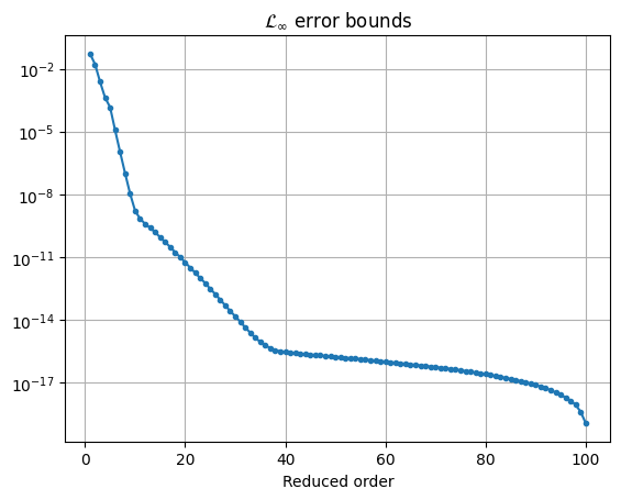
Before we use the reduce method to
obtain a reduced-order model, we take a look at some a priori error bounds for
the reductor. In particular, we get a \(\mathcal{L}_\infty\) rather than the
\(\mathcal{H}_\infty\) error bound from classic balanced truncation.
error_bounds = fdbt.error_bounds()
fig, ax = plt.subplots()
ax.semilogy(range(1, len(error_bounds) + 1), error_bounds, '.-')
ax.set_xlabel('Reduced order')
_ = ax.set_title(r'$\mathcal{L}_\infty$ error bounds')
To get a reduced-order model of order 10, we call the reduce method with the
appropriate argument:
rom = fdbt.reduce(10)
Alternatively, we can specify a desired error tolerance rather than the order of the reduced model.
Finally, we can compute the relative \(\mathcal{L}_\infty\) error to check the quality of the reduced-order model.
err = fom - rom
print(f'Relative Linf error:   {err.linf_norm() / fom.linf_norm():.3e}')
Relative Linf error: 2.980e-09
Clearly, this result is in accordance with our previously computed \(\mathcal{L}_\infty\) error bound:
print(f'Linf error:   {err.linf_norm():.3e}')
print(f'Linf upper bound:   {error_bounds[9]:.3e}')
Linf error:   8.497e-10
Linf upper bound:   1.646e-09
Gap-IRKA
The IRKAReductor is specifically designed to find
\(\mathcal{H}_2\)-optimal reduced-order models (see e.g. [GAB08]).
Since we cannot compute \(\mathcal{H}_2\)-norms for unstable systems,
we can not expect the IRKA to yield high-quality approximations for unstable
full-order models.
In [BBG19] the authors introduce a variant of the IRKA (the Gap-IRKA) which
is based on the \(\mathcal{H}_2\)-gap-norm.
As desired, this norm is defined for most unstable systems which makes the
Gap-IRKA a suitable algorithm for finding reduced-order models for unstable systems.
One major advantage of the GapIRKAReductor over the
FDBTReductor is that
no a priori information about the system poles is required. However, we do not
obtain an a priori \(\mathcal{L}_\infty\) error bound. Let us compute a
reduced-order model of order 10 using the GapIRKAReductor.
from pymor.reductors.h2 import GapIRKAReductor
gapirka = GapIRKAReductor(fom)
rom = gapirka.reduce(10)
Beside the desired order of the reduced model, the reduce method has a few
other arguments as well: conv_crit allows for choosing the stopping criterion
of the algorithm. By specifying conv_crit='sigma' the relative change in
interpolation points, conv_crit='htwogap' the relative change in
\(\mathcal{H}_2\)-gap distance of the reduced-order models and conv_crit='ltwo' the
relative change of \(\mathcal{L}_2\) distances of the reduced-order models are
used as a stopping criterion. The tol argument sets the tolerance for
any of the chosen stopping criterion.
Again, we can compute the relative \(\mathcal{L}_\infty\) error.
err = fom - rom
print(f'Relative Linf error:   {err.linf_norm() / fom.linf_norm():.3e}')
Relative Linf error: 2.849e-09
Download the code:
tutorial_unstable_lti_systems.md,
tutorial_unstable_lti_systems.ipynb.