Run this tutorial

Click here to run this tutorial on binder:
Please note that starting the notebook server may take a couple of minutes.

Tutorial: Reducing an LTI system using balanced truncation

Here we briefly describe the balanced truncation method, for asymptotically stable LTI systems with an invertible \(E\) matrix, and demonstrate it on the heat equation example from Tutorial: Linear time-invariant systems. First, we import necessary packages, including BTReductor.

import matplotlib.pyplot as plt
import numpy as np
import scipy.sparse as sps
from pymor.models.iosys import LTIModel
from pymor.reductors.bt import BTReductor

plt.rcParams['axes.grid'] = True

Then we build the matrices

import numpy as np
import scipy.sparse as sps

k = 50
n = 2 * k + 1

E = sps.eye(n, format='lil')
E[0, 0] = E[-1, -1] = 0.5
E = E.tocsc()

d0 = n * [-2 * (n - 1)**2]
d1 = (n - 1) * [(n - 1)**2]
A = sps.diags([d1, d0, d1], [-1, 0, 1], format='lil')
A[0, 0] = A[-1, -1] = -n * (n - 1)
A = A.tocsc()

B = np.zeros((n, 2))
B[:, 0] = 1
B[0, 0] = B[-1, 0] = 0.5
B[0, 1] = n - 1

C = np.zeros((3, n))
C[0, :n//3] = C[1, n//3:2*n//3] = C[2, 2*n//3:] = 1
C /= C.sum(axis=1)[:, np.newaxis]

and form the full-order model.

fom = LTIModel.from_matrices(A, B, C, E=E)

Balanced truncation

As the name suggests, the balanced truncation method consists of finding a balanced realization of the full-order LTI system and truncating it to obtain a reduced-order model.

The balancing part is based on the fact that a single LTI system has many realizations. For example, starting from a realization

\[\begin{split}\begin{align} E \dot{x}(t) & = A x(t) + B u(t), \\ y(t) & = C x(t) + D u(t), \end{align}\end{split}\]

another realization can be obtained by replacing \(x(t)\) with \(T \tilde{x}(t)\) or by pre-multiplying the differential equation with an invertible matrix. In particular, there exist invertible transformation matrices \(T, S \in \mathbb{R}^{n \times n}\) such that the realization with \(\tilde{E} = S^{\operatorname{T}} E T = I\), \(\tilde{A} = S^{\operatorname{T}} A T\), \(\tilde{B} = S^{\operatorname{T}} B\), \(\tilde{C} = C T\) has Gramians \(\tilde{P}\) and \(\tilde{Q}\) satisfying \(\tilde{P} = \tilde{Q} = \Sigma = \operatorname{diag}(\sigma_i)\), where \(\sigma_i\) are the Hankel singular values (see Tutorial: Linear time-invariant systems for more details). Such a realization is called balanced.

The truncation part is based on the controllability and observability energies. The controllability energy \(E_c(x_0)\) is the minimum energy (squared \(\mathcal{L}_2\) norm of the input) necessary to steer the system from the zero state to \(x_0\). The observability energy \(E_o(x_0)\) is the energy of the output (squared \(\mathcal{L}_2\) norm of the output) for a system starting at the state \(x_0\) and with zero input. It can be shown for the balanced realization (and same for any other realization) that, if \(\tilde{P}\) is invertible, then

\[E_c(x_0) = x_0 \tilde{P}^{-1} x_0, \quad E_o(x_0) = x_0 \tilde{Q} x_0.\]

Therefore, states corresponding to small Hankel singular values are more difficult to reach (they have a large controllability energy) and are difficult to observe (they produce a small observability energy). In this sense, it is then reasonable to truncate these states. This can be achieved by taking as basis matrices \(V, W \in \mathbb{R}^{n \times r}\) the first \(r\) columns of \(T\) and \(S\), possibly after orthonormalization, giving a reduced-order model

\[\begin{split}\begin{align} \hat{E} \dot{\hat{x}}(t) & = \hat{A} \hat{x}(t) + \hat{B} u(t), \\ \hat{y}(t) & = \hat{C} \hat{x}(t) + D u(t), \end{align}\end{split}\]

with \(\hat{E} = W^{\operatorname{T}} E V\), \(\hat{A} = W^{\operatorname{T}} A V\), \(\hat{B} = W^{\operatorname{T}} B\), \(\hat{C} = C V\).

It is known that the reduced-order model is asymptotically stable if \(\sigma_r > \sigma_{r + 1}\). Furthermore, it satisfies the \(\mathcal{H}_\infty\) error bound

\[\lVert H - \hat{H} \rVert_{\mathcal{H}_\infty} \leqslant 2 \sum_{i = r + 1}^n \sigma_i.\]

Note that any reduced-order model (not only from balanced truncation) satisfies the lower bound

\[\lVert H - \hat{H} \rVert_{\mathcal{H}_\infty} \geqslant \sigma_{r + 1}.\]

Balanced truncation in pyMOR

To run balanced truncation in pyMOR, we first need the reductor object

bt = BTReductor(fom)

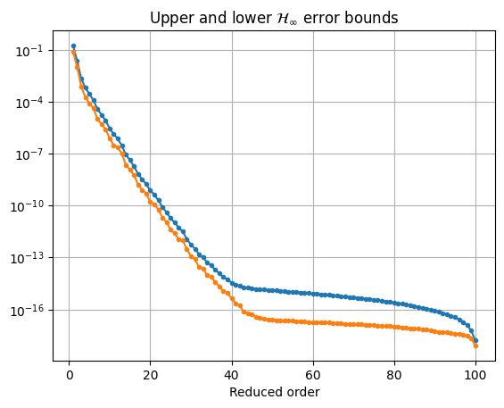
Calling its reduce method runs the balanced truncation algorithm. This reductor additionally has an error_bounds method which can compute the a priori \(\mathcal{H}_\infty\) error bounds based on the Hankel singular values:

error_bounds = bt.error_bounds()
hsv = fom.hsv()
fig, ax = plt.subplots()
ax.semilogy(range(1, len(error_bounds) + 1), error_bounds, '.-')
ax.semilogy(range(1, len(hsv)), hsv[1:], '.-')
ax.set_xlabel('Reduced order')
_ = ax.set_title(r'Upper and lower $\mathcal{H}_\infty$ error bounds')

To get a reduced-order model of order 10, we call the reduce method with the appropriate argument:

rom = bt.reduce(10)

Instead, or in addition, a tolerance for the \(\mathcal{H}_\infty\) error can be specified, as well as the projection algorithm (by default, the balancing-free square root method is used). The used Petrov-Galerkin bases are stored in bt.V and bt.W.

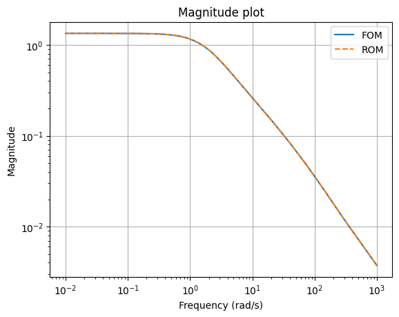
We can compare the magnitude plots between the full-order and reduced-order models

w = (1e-2, 1e3)
fig, ax = plt.subplots()
fom.transfer_function.mag_plot(w, ax=ax, label='FOM')
rom.transfer_function.mag_plot(w, ax=ax, linestyle='--', label='ROM')
_ = ax.legend()

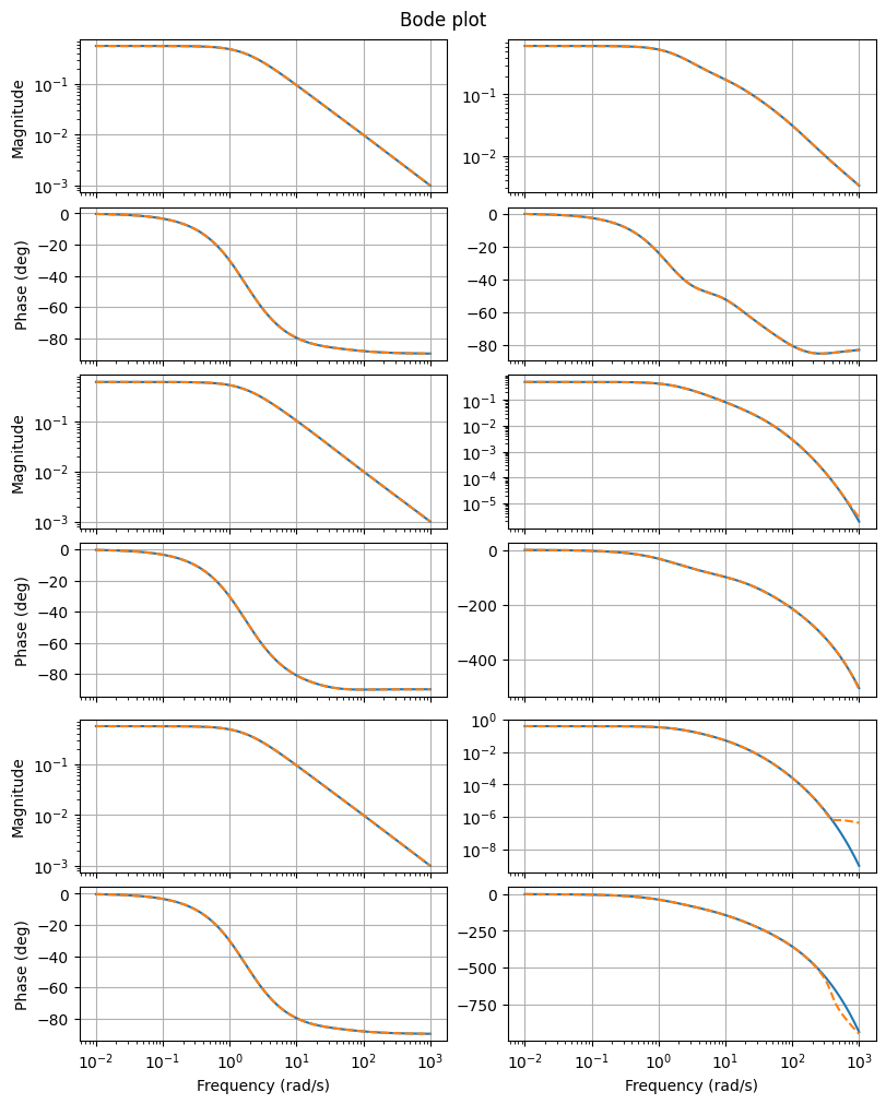
as well as Bode plots

fig, axs = plt.subplots(6, 2, figsize=(8, 10), sharex=True, constrained_layout=True)
fom.transfer_function.bode_plot(w, ax=axs)
_ = rom.transfer_function.bode_plot(w, ax=axs, linestyle='--')

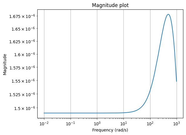
Also, we can plot the magnitude plot of the error system, which is again an LTI system.

\[\begin{split}\begin{align} \begin{bmatrix} E & 0 \\ 0 & \hat{E} \end{bmatrix} \begin{bmatrix} \dot{x}(t) \\ \dot{\hat{x}}(t) \end{bmatrix} & = \begin{bmatrix} A & 0 \\ 0 & \hat{A} \end{bmatrix} \begin{bmatrix} x(t) \\ \hat{x}(t) \end{bmatrix} + \begin{bmatrix} B \\ \hat{B} \end{bmatrix} u(t), \\ y(t) - \hat{y}(t) & = \begin{bmatrix} C & -\hat{C} \end{bmatrix} \begin{bmatrix} x(t) \\ \hat{x}(t) \end{bmatrix}. \end{align}\end{split}\]

err = fom - rom
_ = err.transfer_function.mag_plot(w)

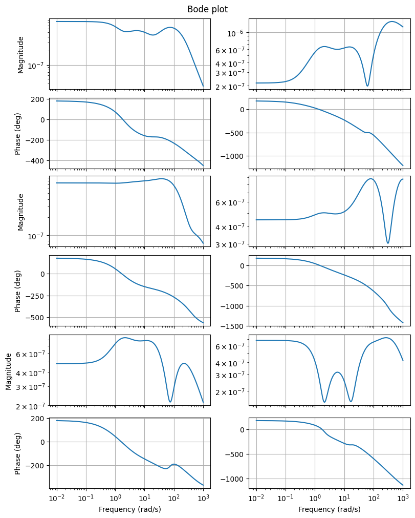
and its Bode plot

fig, axs = plt.subplots(6, 2, figsize=(8, 10), sharex=True, constrained_layout=True)
_ = err.transfer_function.bode_plot(w, ax=axs)

Finally, we can compute the relative errors in different system norms.

print(f'Relative Hinf error:   {err.hinf_norm() / fom.hinf_norm():.3e}')
print(f'Relative H2 error:     {err.h2_norm() / fom.h2_norm():.3e}')
print(f'Relative Hankel error: {err.hankel_norm() / fom.hankel_norm():.3e}')

Relative Hinf error:   1.236e-06
Relative H2 error:     6.797e-05

Relative Hankel error: 2.377e-06

Download the code: tutorial_bt.md, tutorial_bt.ipynb.