Tutorial: Building a Reduced Basis
Run this tutorial
Click here to run this tutorial on mybinder.org:In this tutorial we will learn more about VectorArrays and how to
construct a reduced basis using pyMOR.
A reduced basis spans a low dimensional subspace of a Model’s
solution_space, in which the
solutions of the Model
can be well approximated for all parameter values. In this context,
time is treated as an additional parameter. So for time-dependent problems,
the reduced space (the span of the reduced basis) should approximate the
solution for all parameter values and time instances.
An upper bound for the possible quality of a reduced space is given by the so-called Kolmogorov \(N\)-width \(d_N\) given as
In this formula \(V\) denotes the
solution_space, \(\mathcal{P} \subset \mathbb{R}^p\)
denotes the set of all parameter values we are interested in, and
\(u(\mu)\) denotes the solution
of the Model for the given parameter values \(\mu\).
In pyMOR the set \(\mathcal{P}\) is called the ParameterSpace.
How to read this formula? For each candidate reduced space \(V_N\) we
look at all possible parameter values \(\mu\) and compute the best-approximation
error in \(V_N\) (the second infimum). The supremum over the infimum
is thus the worst-case best-approximation error over all parameter values of
interest. Now we take the infimum of the worst-case best-approximation errors
over all possible reduced spaces of dimension at most \(N\), and this is
\(d_N\).
So whatever reduced space of dimension \(N\) we pick, we will always find a \(\mu\) for which the best-approximation error in our space is at least \(d_N\). Reduced basis methods aim at constructing spaces \(V_N\) for which the worst-case best-approximation error is as close to \(d_N\) as possible.
However, we will only find a good \(V_N\) of small dimension \(N\) if the values \(d_N\) decrease quickly for growing \(N\). It can be shown that this is the case as soon as \(u(\mu)\) analytically depends on \(\mu\), which is true for many problems of interest. More precisely, it can be shown [BCDDPW11], [DPW13] that there are constants \(C, c > 0\) such that
In this tutorial we will construct reduced spaces \(V_N\) for a concrete problem with pyMOR and study their error decay.
Model setup
First we need to define a Model and a ParameterSpace for which we want
to build a reduced basis. We choose here the standard
thermal block benchmark
problem shipped with pyMOR (see Getting started). However, any pyMOR
Model can be used, except for Section ‘Weak greedy algorithm’ where
some more assumptions have to be made on the Model.
First we import everything we need:
import numpy as np
from pymor.basic import *
Then we build a 3-by-3 thermalblock problem that we discretize using pyMOR’s
builtin discretizers (see
Tutorial: Using pyMOR’s discretization toolkit for an introduction to pyMOR’s discretization toolkit).
problem = thermal_block_problem((3,3))
fom, _ = discretize_stationary_cg(problem, diameter=1/100)
Next, we need to define a ParameterSpace of parameter values for which
the solutions of the full-order model fom should be approximated by the reduced basis.
We do this by calling the space method
of the Parameters of fom:
parameter_space = fom.parameters.space(0.0001, 1.)
Here, 0.0001 and 1. are the common lower and upper bounds for the
individual components of all Parameters of fom. In our case fom
expects a single parameter 'diffusion' of 9 values:
fom.parameters
Parameters({diffusion: 9})
If fom were to depend on multiple Parameters, we could also call the
space method with a dictionary
of lower and upper bounds per parameter.
The main use of ParameterSpaces in pyMOR is that they allow to easily sample
parameter values from their domain using the methods
sample_uniformly and
sample_randomly.
Computing the snapshot data
Reduced basis methods are snapshot-based, which means that they build
the reduced space as a linear subspace of the linear span of solutions
of the fom for certain parameter values. The easiest
approach is to just pick these values randomly, what we will do in the
following. First we define a training set of 25 parameters:
training_set = parameter_space.sample_randomly(25)
print(training_set)
[Mu({diffusion: [0.37460266483547777, 0.9507192349792751, 0.7320207424172239, 0.5986986183486169, 0.15610303857839228, 0.15607892088416903, 0.05817780380698265, 0.8661895281603577, 0.6011549002420344]}), Mu({diffusion: [0.7081017705382658, 0.020682435846372867, 0.9699128611767781, 0.8324593965363417, 0.21241787676720833, 0.1819067847103799, 0.18348616940244847, 0.30431181873524177, 0.5248039559890746]}), Mu({diffusion: [0.43200182414025157, 0.2913000172840221, 0.6118917094329073, 0.13957991126597663, 0.2922154340703646, 0.3664252071093623, 0.4561243772186142, 0.7851974437968743, 0.1997538147801439]}), Mu({diffusion: [0.5142830149697702, 0.5924553274051563, 0.04654576767872573, 0.6075840974162482, 0.17060707127492278, 0.065145087825981, 0.9488906486996079, 0.9656354698712519, 0.8084165083816495]}), Mu({diffusion: [0.30468330779645336, 0.09776234679498323, 0.6842646032095057, 0.4402084784902273, 0.12212603102129435, 0.49522739242025904, 0.03448508226310688, 0.9093294700385742, 0.2588541036018569]}), Mu({diffusion: [0.6625560321255466, 0.311779904981802, 0.520116014375693, 0.5467556083153453, 0.18493597007997448, 0.9695876693017821, 0.7751553100787785, 0.9395049916700327, 0.8948378676926061]}), Mu({diffusion: [0.597940188813204, 0.9218820475996146, 0.0885836528017143, 0.1960632641329033, 0.04532276618164702, 0.325397797730188, 0.38873842196051306, 0.2714218968707185, 0.8287546354010141]}), Mu({diffusion: [0.3568176513609199, 0.28100641623641204, 0.5427418135499327, 0.14101013255226516, 0.8022167610559643, 0.07464318861540285, 0.9868882479068573, 0.7722675448197277, 0.19879580996601898]}), Mu({diffusion: [0.005621564911890039, 0.8154798823119886, 0.7068866581132324, 0.7290342673241832, 0.7712932196512772, 0.07413724726891696, 0.35852988197141816, 0.1159574726191772, 0.863117115533006]}), Mu({diffusion: [0.6233357970148752, 0.3309649350501639, 0.06365199445099504, 0.3110512234834906, 0.32525080369454434, 0.7296332177202303, 0.6375937156080776, 0.8872240213020689, 0.4722677036694331]}), Mu({diffusion: [0.11968228651370788, 0.7132734627442727, 0.7608089701120357, 0.5613210698497393, 0.7709900832365655, 0.4938462168047543, 0.5227805560990558, 0.42759826425671377, 0.025516584831420778]}), Mu({diffusion: [0.10798063785060512, 0.031526042768165584, 0.6364467702226541, 0.314424545478219, 0.5086198340955863, 0.9075757172787005, 0.24936729992596005, 0.41044188474332616, 0.7555755834291944]}), Mu({diffusion: [0.2288752856750733, 0.07707221183781011, 0.28982247776847664, 0.161305165125279, 0.9297046825773388, 0.8081395675264605, 0.6334404161347724, 0.871473444128699, 0.8036917096914246]}), Mu({diffusion: [0.18665140188014723, 0.8925697425901288, 0.5393883076914592, 0.8074594111485461, 0.8961016907935009, 0.3180716746243667, 0.11014091933522399, 0.22801236902568747, 0.42716507784739366]}), Mu({diffusion: [0.8180329644459009, 0.8607445101980178, 0.007051435318137585, 0.5107962278473079, 0.41746926204846413, 0.22218559968968316, 0.11995338079694944, 0.3376814098864876, 0.9429154129421279]}), Mu({diffusion: [0.32327061172755317, 0.5188387426811918, 0.7030486569992883, 0.36369323941905607, 0.9717849045126886, 0.962451050212617, 0.2518571175957816, 0.4972987810417962, 0.30094822198578797]}), Mu({diffusion: [0.2849120103280299, 0.03698325865979735, 0.6096033775464988, 0.5027287553265386, 0.05157360337486436, 0.27871859959018774, 0.9082750593780571, 0.2396379344779057, 0.14498038260401397]}), Mu({diffusion: [0.4895038150015352, 0.9856518890651896, 0.24213106598434925, 0.672168333851138, 0.7616434533671848, 0.2377137802380004, 0.7282435269769983, 0.3678463544059813, 0.6323426000105201]}), Mu({diffusion: [0.6335663577898186, 0.535821106606351, 0.09038074107740286, 0.8353189653396791, 0.32084798696523864, 0.18659985854881422, 0.040871064040608446, 0.590933853893923, 0.6775966054060982]}), Mu({diffusion: [0.016686170144963364, 0.512141848993451, 0.22657312562041815, 0.645208273130409, 0.17444899236209094, 0.6909686443286557, 0.38679667276590735, 0.9367363157378609, 0.13760719205157865]}), Mu({diffusion: [0.3411322444151535, 0.11356217388846501, 0.9247011489167349, 0.8773516194456429, 0.2580158335523841, 0.6600180476295756, 0.8172404779811957, 0.5552452915183024, 0.5296976132981709]}), Mu({diffusion: [0.24192810567136164, 0.09319345752911863, 0.8972260363775314, 0.9004280153576141, 0.6331381471275406, 0.3390958880695958, 0.3492746536551996, 0.7259830833023524, 0.8971205489265819]}), Mu({diffusion: [0.8870977156226908, 0.7798975583030381, 0.6420674429896723, 0.08423155099854933, 0.1617125512232043, 0.8985643331082266, 0.606468416753624, 0.009296131911467984, 0.10156139571174551]}), Mu({diffusion: [0.663535418931145, 0.005161077687834065, 0.16089197061235688, 0.5487789159876495, 0.6919260081729239, 0.6519960633766503, 0.2243468825296137, 0.7122080034254011, 0.23732536258805037]}), Mu({diffusion: [0.32546715818945177, 0.7465167559775123, 0.64966793575731, 0.8492384881531285, 0.6576471310111133, 0.568351772475138, 0.09376540035130967, 0.36777903147912755, 0.26527584744495725]})]
Then we solve the full-order model
for all parameter values in the training set and accumulate all
solution vectors in a single VectorArray using its
append method. But first
we need to create an empty VectorArray to which the solutions can
be appended. New VectorArrays in pyMOR are always created by a
corresponding VectorSpace. Empty arrays are created using the
empty method. But what
is the right VectorSpace? All solutions
of a Model belong to its solution_space,
so we write:
U = fom.solution_space.empty()
for mu in training_set:
    U.append(fom.solve(mu))
Note that fom.solve returns a VectorArray containing a single vector.
This entire array (of one vector) is then appended to the U array.
pyMOR has no notion of single vectors, we only speak of VectorArrays.
What exactly is a VectorSpace? A VectorSpace in pyMOR holds all
information necessary to build VectorArrays containing vector objects
of a certain type. In our case we have
fom.solution_space
NumpyVectorSpace(20201, id='STATE')
which means that the created VectorArrays will internally hold
NumPy arrays for data storage. The number is the dimension of the
vector. We have here a NumpyVectorSpace because pyMOR’s builtin
discretizations are built around the NumPy/SciPy stack. If fom would
represent a Model living in an external PDE solver, we would have
a different type of VectorSpace which, for instance, might hold a
reference to a discrete functions space object inside the PDE solver
instead of the dimension.
After appending all solutions vectors to U, we can verify that U
now really contains 25 vectors:
len(U)
25
Note that appending one VectorArray V to another array U
will append copies of the vectors in V to U. So
modifying U will not affect V.
Let’s look at the solution snapshots we have just computed using
the visualize method of fom.
A VectorArray containing multiple vectors is visualized as a
time series:
fom.visualize(U)
A trivial reduced basis
Given some snapshot data, the easiest option to get a reduced basis is to just use the snapshot vectors as the basis:
trivial_basis = U.copy()
Note that assignment in Python never copies data! Thus, if we had written
trivial_basis = U and modified trivial_basis, U would change
as well, since trivial_basis and U would refer to the same
VectorArray object. So whenever you want to use one VectorArray
somewhere else and you are unsure whether some code might change the
array, you should always create a copy. pyMOR uses copy-on-write semantics
for copies of VectorArrays, which means that generally calling
copy is cheap as it does
not duplicate any data in memory. Only when you modify one of the arrays
the data will be copied.
Now we want to know how good our reduced basis is. So we want to compute
where \(V_N\) denotes the span of our reduced basis, for all
\(\mu\) in some validation set of parameter values. Assuming that
we are in a Hilbert space, we can compute the infimum via orthogonal
projection onto \(V_N\): in that case, the projection will be the
best approximation in \(V_N\) and the norm of the difference between
\(u(\mu)\) and its orthogonal projection will be the best-approximation
error.
So let \(v_{proj}\) be the orthogonal projection of \(v\) onto the linear space spanned by the basis vectors \(u_i,\ i=1, \ldots, N\). By definition this means that \(v - v_{proj}\) is orthogonal to all \(u_i\):
Let \(\lambda_j\), \(j = 1, \ldots, N\) be the coefficients of \(v_{proj}\) with respect to this basis, i.e. \(\sum_{j=1}^N \lambda_j u_j = v_{proj}\). Then:
With \(G_{i,j} := (u_i, u_j)\), \(R := [(v, u_1), \ldots, (v, u_N)]^T\) and \(\Lambda := [\lambda_1, \ldots, \lambda_N]^T\), we obtain the linear equation system
which determines \(\lambda_i\) and, thus, \(v_{proj}\).
Let’s assemble and solve this equation system using pyMOR to determine
the best-approximation error in trivial_basis for some test vector
V which we take as another random solution of our Model:
V = fom.solve(parameter_space.sample_randomly(1)[0])
The matrix \(G\) of all inner products between vectors in trivial_basis
is a so called Gramian matrix.
Consequently, every VectorArray has a gramian method, which computes precisely
this matrix:
G = trivial_basis.gramian()
The Gramian is computed w.r.t. the Euclidean inner product. For the
right-hand side \(R\), we need to compute all (Euclidean) inner
products between the vectors in trivial_basis and (the single vector in)
V. For that, we can use the inner
method:
R = trivial_basis.inner(V)
which will give us a \(25\times 1\) NumPy array of all inner products.
Now, we can use NumPy to solve the linear equation system:
lambdas = np.linalg.solve(G, R)
Finally, we need to form the linear combination
using the lincomb method
of trivial_basis. It expects row vectors of linear coefficients, but
solve returns column vectors, so we need to take the transpose:
V_proj = trivial_basis.lincomb(lambdas.T)
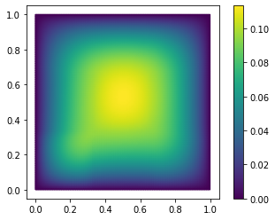
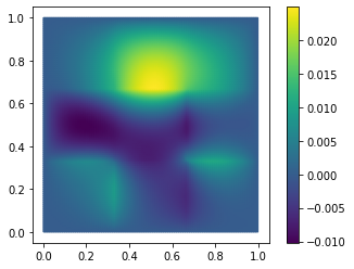
Let’s look at V, V_proj and the difference of both. VectorArrays of
the same length can simply be subtracted, yielding a new array of the
differences:
fom.visualize((V, V_proj, V - V_proj),
              legend=('V', 'V_proj', 'best-approximation err'),
              separate_colorbars=True)

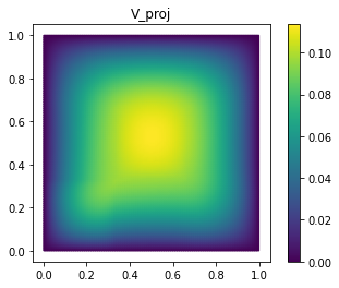
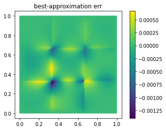
As you can see, we already have a quite good approximation of V with
only 25 basis vectors.
Now, the Euclidean norm will just work fine in many cases. However, when the full-order model comes from a PDE, it will be usually not the norm we are interested in, and you may get poor results for problems with strongly anisotropic meshes.
For our diffusion problem with homogeneous Dirichlet boundaries,
the Sobolev semi-norm (of order one) is a natural choice. Among other useful products,
discretize_stationary_cg already
assembled a corresponding inner product Operator for us, which is available
as
fom.h1_0_semi_product
NumpyMatrixOperator(<20201x20201 sparse, 140601 nnz>, source_id='STATE', range_id='STATE', name='h1_0_semi')
Note
The 0 in h1_0_semi_product refers to the fact that rows and columns of
Dirichlet boundary DOFs have been cleared in the matrix of the Operator to
make it invertible. This is important for being able to compute Riesz
representatives w.r.t. this inner product (required for a posteriori
estimation of the ROM error). If you want to compute the H1 semi-norm of a
function that does not vanish at the Dirichlet boundary, use
fom.h1_semi_product.
To use fom.h1_0_semi_product as an inner product Operator for computing the
projection error, we can simply pass it as the optional product argument to
gramian and
inner:
G = trivial_basis[:10].gramian(product=fom.h1_0_semi_product)
R = trivial_basis[:10].inner(V, product=fom.h1_0_semi_product)
lambdas = np.linalg.solve(G, R)
V_h1_proj = trivial_basis[:10].lincomb(lambdas.T)

fom.visualize((V, V_h1_proj, V - V_h1_proj), separate_colorbars=True)
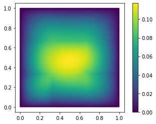
As you might have guessed, we have additionally opted here to only use the
span of the first 10 basis vectors of trivial_basis. Like NumPy arrays,
VectorArrays can be sliced and indexed. The result is always a
view onto the
original data. If the view object is modified, the original array is modified
as well.
Next we will assess the approximation error a bit more thoroughly, by
evaluating it on a validation set of 100 parameter values for varying
basis sizes.
First, we compute the validation snapshots:
validation_set = parameter_space.sample_randomly(100)
V = fom.solution_space.empty()
for mu in validation_set:
    V.append(fom.solve(mu))
To optimize the computation of the projection matrix and the right-hand side for varying basis sizes, we first compute these for the full basis and then extract appropriate sub-matrices:
def compute_proj_errors(basis, V, product):
    G = basis.gramian(product=product)
    R = basis.inner(V, product=product)
    errors = []
    for N in range(len(basis) + 1):
        if N > 0:
            v = np.linalg.solve(G[:N, :N], R[:N, :])
        else:
            v = np.zeros((0, len(V)))
        V_proj = basis[:N].lincomb(v.T)
        errors.append(np.max((V - V_proj).norm(product=product)))
    return errors

trivial_errors = compute_proj_errors(trivial_basis, V, fom.h1_0_semi_product)
Here we have used the fact that we can form multiple linear combinations at once by passing
multiple rows of linear coefficients to
lincomb. The
norm method returns a
NumPy array of the norms of all vectors in the array with respect to
the given inner product Operator. When no norm is specified, the Euclidean
norms of the vectors are computed.
Let’s plot the projection errors:
from matplotlib import pyplot as plt
plt.figure()
plt.semilogy(trivial_errors)
plt.ylim(1e-1, 1e1)
plt.show()
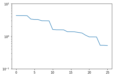
Good! We see an exponential decay of the error with growing basis size. However, we can do better. If we want to use a smaller basis than we have snapshots available, just picking the first of these obviously won’t be optimal.
Strong greedy algorithm
The strong greedy algorithm iteratively builds reduced spaces \(V_N\) with a small worst-case best approximation error on a training set of solution snapshots by adding, in each iteration, the currently worst-approximated snapshot vector to the basis of \(V_N\).
We can easily implement it as follows:
def strong_greedy(U, product, N):
    basis = U.space.empty()

    for n in range(N):
        # compute projection errors
        G = basis.gramian(product)
        R = basis.inner(U, product=product)
        lambdas = np.linalg.solve(G, R)
        U_proj = basis.lincomb(lambdas.T)
        errors = (U - U_proj).norm(product)

        # extend basis
        basis.append(U[np.argmax(errors)])

    return basis
Obviously, this algorithm is not optimized as we keep computing inner products we already know, but it will suffice for our purposes. Let’s compute a reduced basis using the strong greedy algorithm:
greedy_basis = strong_greedy(U, fom.h1_0_product, 25)
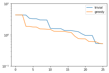
We compute the approximation errors for the validation set as before:
greedy_errors = compute_proj_errors(greedy_basis, V, fom.h1_0_semi_product)

plt.figure()
plt.semilogy(trivial_errors, label='trivial')
plt.semilogy(greedy_errors, label='greedy')
plt.ylim(1e-1, 1e1)
plt.legend()
plt.show()

Indeed, the strong greedy algorithm constructs better bases than the trivial basis construction algorithm. For compact training sets contained in a Hilbert space, it can actually be shown that the greedy algorithm constructs quasi-optimal spaces in the sense that polynomial or exponential decay of the N-widths \(d_N\) yields similar rates for the worst-case best-approximation errors of the constructed \(V_N\).
Orthonormalization required
There is one technical problem with both algorithms however: the condition numbers of the Gramians used to compute the projection onto \(V_N\) explode:
G_trivial = trivial_basis.gramian(fom.h1_0_semi_product)
G_greedy = greedy_basis.gramian(fom.h1_0_semi_product)
trivial_conds, greedy_conds = [], []
for N in range(1, len(U)):
    trivial_conds.append(np.linalg.cond(G_trivial[:N, :N]))
    greedy_conds.append(np.linalg.cond(G_greedy[:N, :N]))
plt.figure()
plt.semilogy(range(1, len(U)), trivial_conds, label='trivial')
plt.semilogy(range(1, len(U)), greedy_conds, label='greedy')
plt.legend()
plt.show()
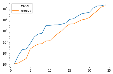
This is quite obvious as the snapshot matrix U becomes more and
more linear dependent the larger it grows.
If we would use the bases we just constructed to build a reduced-order model from them, we will quickly get bitten by the limited accuracy of floating-point numbers.
There is a simple remedy however: we orthonormalize our bases. The standard
algorithm in pyMOR to do so, is a modified
gram_schmidt procedure with
re-orthogonalization to improve numerical accuracy:
gram_schmidt(greedy_basis, product=fom.h1_0_semi_product, copy=False)
gram_schmidt(trivial_basis, product=fom.h1_0_semi_product, copy=False)
The copy=False argument tells the algorithm to orthonormalize
the given VectorArray in-place instead of returning a new array with
the orthonormalized vectors.
Since the vectors in greedy_basis and trivial_basis are now orthonormal,
their Gramians are identity matrices (up to numerics). Thus, their condition
numbers should be near 1:
G_trivial = trivial_basis.gramian(fom.h1_0_semi_product)
G_greedy = greedy_basis.gramian(fom.h1_0_semi_product)

print(f'trivial: {np.linalg.cond(G_trivial)}, '
      f'greedy: {np.linalg.cond(G_greedy)}')
trivial: 1.0000000000000038, greedy: 1.000000000000002
Orthonormalizing the bases does not change their linear span, so best-approximation errors stay the same. Also, we can compute these errors now more easily by exploiting orthogonality:
def compute_proj_errors_orth_basis(basis, V, product):
    errors = []
    for N in range(len(basis) + 1):
        v = V.inner(basis[:N], product=product)
        V_proj = basis[:N].lincomb(v)
        errors.append(np.max((V - V_proj).norm(product)))
    return errors

trivial_errors = compute_proj_errors_orth_basis(trivial_basis, V, fom.h1_0_semi_product)
greedy_errors  = compute_proj_errors_orth_basis(greedy_basis, V, fom.h1_0_semi_product)

plt.figure()
plt.semilogy(trivial_errors, label='trivial')
plt.semilogy(greedy_errors, label='greedy')
plt.ylim(1e-1, 1e1)
plt.legend()
plt.show()
Proper Orthogonal Decomposition
Another popular method to create a reduced basis out of snapshot data is the so-called Proper Orthogonal Decomposition (POD) which can be seen as a non-centered version of Principal Component Analysis (PCA). First we build a snapshot matrix
where \(K\) denotes the total number of solution snapshots. Then we compute the SVD of \(A\)
where \(\Sigma\) is an \(r \times r\)-diagonal matrix, \(U\) is an \(n \times r\)-matrix
and \(V\) is an \(K \times r\)-matrix. Here \(n\) denotes the dimension of the
solution_space and \(r\) is the rank of \(A\).
The diagonal entries \(\sigma_i\) of \(\Sigma\) are the singular values of \(A\), which are
assumed to be monotonically decreasing. The pairwise orthogonal and normalized
columns of \(U\) and \(V\) are the left- resp. right-singular vectors of \(A\).
The \(i\)-th POD mode is than simply the \(i\)-th left-singular vector of \(A\),
i.e. the \(i\)-th column of \(U\). The larger the corresponding singular value is,
the more important is this vector for the approximation of the snapshot data. In fact, if we
let \(V_N\) be the span of the first \(N\) left-singular vectors of \(A\), then
the following error identity holds:
Thus, the linear spaces produced by the POD are actually optimal, albeit in a different
error measure: instead of looking at the worst-case best-approximation error over all
parameter values, we minimize the \(\ell^2\)-sum of all best-approximation errors.
So in the mean squared average, the POD spaces are optimal, but there might be parameter values
for which the best-approximation error is quite large.
So far we completely neglected that the snapshot vectors may lie in a Hilbert space
with some given inner product. To account for that, instead of the snapshot matrix
\(A\), we consider the linear mapping that sends the \(i\)-th canonical basis vector
\(e_k\) of \(\mathbb{R}^K\) to the vector \(u(\mu_k)\) in the
solution_space:
Also for this finite-rank (hence compact) operator there exists a SVD of the form
with orthonormal vectors \(u_i\) and \(v_i\) that generalizes the SVD of a matrix.
The POD in this more general form is implemented in pyMOR by the
pod method, which can be called as follows:
pod_basis, pod_singular_values = pod(U, product=fom.h1_0_semi_product, modes=25)
We said that the POD modes (left-singular vectors) are orthonormal with respect to the inner product on the target Hilbert-space. Let’s check that:
np.linalg.cond(pod_basis.gramian(fom.h1_0_semi_product))
1.000000000010063
Now, let us compare how the POD performs against the greedy algorithm in the worst-case best-approximation error:
pod_errors = compute_proj_errors_orth_basis(pod_basis, V, fom.h1_0_semi_product)

plt.figure()
plt.semilogy(trivial_errors, label='trivial')
plt.semilogy(greedy_errors, label='greedy')
plt.semilogy(pod_errors, label='POD')
plt.ylim(1e-1, 1e1)
plt.legend()
plt.show()
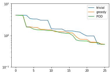
As it turns out, the POD spaces perform even slightly better than the greedy spaces. Why is that the case? Note that for finite training or validation sets, both considered error measures are equivalent. In particular:
Since POD spaces are optimal in the \(\ell^2\)-error, they miss the error of the optimal space in the Kolmogorov sense by at most a factor of \(\sqrt{K}\), which in our case is \(5\). On the other hand, the greedy algorithm also only produces quasi-optimal spaces. – For very large training sets with more complex parameter dependence, differences between both spaces may be more significant.
Finally, it is often insightful to look at the POD modes themselves:
fom.visualize(pod_basis)
As you can see, the first (more important) basis vectors account for the approximation of the solutions in the bulk of the subdomains, whereas the higher modes are responsible for approximating the solutions at the subdomain interfaces.
Weak greedy algorithm
Both POD and the strong greedy algorithm require the computation of all
solutions \(u(\mu)\)
for all parameter values \(\mu\) in the training_set. So it is
clear right from the start that we cannot afford very large training sets.
Otherwise we would not be interested in model order reduction
in the first place. This is a problem when the number of Parameters
increases and/or the solution depends less uniformly on the Parameters.
Reduced basis methods have a very elegant solution to this problem, which allows training sets that are orders of magnitude larger than the training sets affordable for POD: instead of computing the best-approximation error we only compute a surrogate
for it. Replacing the best-approximation error by this surrogate in the
strong greedy algorithm, we arrive at the
weak greedy
algorithm. If the surrogate \(\mathcal{E}(\mu)\) is an upper and lower bound
to the best-approximation error up to some fixed factor, it can still be shown that the
produced reduced spaces are quasi-optimal in the same sense as for the strong greedy
algorithm, although the involved constants might be worse, depending on the
efficiency of \(\mathcal{E}(\mu)\).
Now here comes the trick: to get a surrogate that can be quickly computed, we can use our current reduced-order model for it. More precisely, we choose \(\mathcal{E}(\mu)\) to be of the form
So to compute the surrogate for fixed parameter values \(\mu\), we first
solve the reduced-order model for the current
reduced basis for these parameter values and then compute an estimate for the
model order reduction error.
We won’t go into any further details in this tutorial, but for nice problem classes
(linear coercive problems with an affine dependence of the system matrix on the Parameters),
one can derive a posteriori error estimators for which the equivalence with the best-approximation
error can be shown and which can be computed efficiently, independently from the size
of the full-order model. Here we will only give a simple example how to use the
weak greedy algorithm for our problem at hand.
In order to do so, we need to be able to build a reduced-order
model with an appropriate error estimator. For the given (linear coercive) thermal block problem
we can use CoerciveRBReductor:
reductor = CoerciveRBReductor(
    fom,
    product=fom.h1_0_semi_product,
    coercivity_estimator=ExpressionParameterFunctional('min(diffusion)', fom.parameters)
)
Here product specifies the inner product with respect to which we want to compute the
model order reduction error. With coercivity_estimator we need to specify
a function which estimates the coercivity constant of the system matrix with respect to
the given inner product. In our case, this is just the minimum of the diffusivities over
all subdomains.
Now we can call rb_greedy, which constructs for us the
surrogate \(\mathcal{E}(\mu)\) from fom and the reductor we just
constructed. It then passes this surrogate to the weak_greedy
method. Furthermore, we need to specify the number of basis vectors we want to compute
(we could also have specified an error tolerance) and the training set.
As the surrogate is cheap to evaluate, we choose here a training set of 1000 different
parameter values:
greedy_data = rb_greedy(fom, reductor, parameter_space.sample_randomly(1000),
                        max_extensions=25)
Take a look at the log output to see how the basis is built iteratively using the surrogate \(\mathcal{E}(\mu)\).
The returned greedy_data dictionary contains various information about the run
of the algorithm, including the final ROM. Here, however, we are interested in the
generated reduced basis, which is managed by the reductor:
weak_greedy_basis = reductor.bases['RB']
Let’s see, how the weak-greedy basis performs:
weak_greedy_errors = compute_proj_errors_orth_basis(weak_greedy_basis, V, fom.h1_0_semi_product)

plt.figure()
plt.semilogy(trivial_errors, label='trivial')
plt.semilogy(greedy_errors, label='greedy')
plt.semilogy(pod_errors, label='POD')
plt.semilogy(weak_greedy_errors, label='weak greedy')
plt.ylim(1e-1, 1e1)
plt.legend()
plt.show()
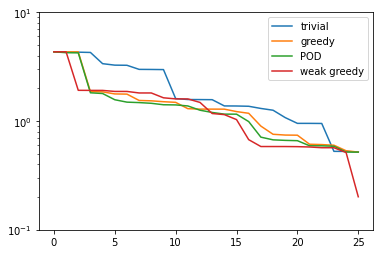
We see that for smaller basis sizes the weak-greedy basis is slightly worse than the POD and
strong-greedy bases. This can be explained by the fact that the surrogate \(\mathcal{E}(\mu)\)
can over-estimate the actual best-approximation error by a certain (fixed) factor, possibly
resulting in the selection of sub-optimal snapshots. For larger basis sizes, this is mitigated
by the very large training set from which we were able to choose: the 25 snapshots in training_set used
for the POD and strong-greedy bases can approximate the entire manifold of solutions only to
a certain degree, whereas the weak-greedy algorithm could select the snapshots from 1000 possible
parameter values.
Download the code:
tutorial_basis_generation.py
tutorial_basis_generation.ipynb