Tutorial: Linear time-invariant systems
Run this tutorial
Click here to run this tutorial on mybinder.org:In this tutorial, we discuss finite-dimensional, continuous-time, linear time-invariant (LTI) systems of the form
where
\(u\) is the input,
\(x\) the state, and
\(y\) the output of the system,
and \(A, B, C, D, E\) are matrices of appropriate dimensions
(more details can be found in [A05]).
In pyMOR, these models are captured by LTIModels,
which contain the matrices \(A, B, C, D, E\) as Operators.
We start by building an LTIModel and then demonstrate some of its properties,
using a discretized heat equation as the example.
We focus on a non-parametric example,
but parametric LTI systems can be handled similarly
by constructing \(A, B, C, D, E\) as parametric Operators and
passing parameter values via the mu argument to the methods of the
LTIModel.
Building a model
We consider the following one-dimensional heat equation over \((0, 1)\) with two inputs \(u_1, u_2\) and three outputs \(y_1, y_2, y_2\):
There are many ways of building an LTIModel.
Here, we show how to build one from custom matrices,
instead of using a discretizer as in Tutorial: Using pyMOR’s discretization toolkit
(and the to_lti method of
InstationaryModel to obtain an LTIModel).
In particular, we will use the
from_matrices method of LTIModel,
which instantiates an LTIModel from NumPy or SciPy matrices.
First, we do the necessary imports and some matplotlib style choices.
import matplotlib.pyplot as plt
import numpy as np
import scipy.sparse as sps
from pymor.models.iosys import LTIModel

plt.rcParams['axes.grid'] = True
Next, we can assemble the matrices based on a centered finite difference approximation using standard methods of NumPy and SciPy.
k = 50
n = 2 * k + 1

E = sps.eye(n, format='lil')
E[0, 0] = E[-1, -1] = 0.5
E = E.tocsc()

d0 = n * [-2 * (n - 1)**2]
d1 = (n - 1) * [(n - 1)**2]
A = sps.diags([d1, d0, d1], [-1, 0, 1], format='lil')
A[0, 0] = A[-1, -1] = -n * (n - 1)
A = A.tocsc()

B = np.zeros((n, 2))
B[:, 0] = 1
B[0, 0] = B[-1, 0] = 0.5
B[0, 1] = n - 1

C = np.zeros((3, n))
C[0, 0] = C[1, k] = C[2, -1] = 1
Then, we can create an LTIModel from NumPy and SciPy matrices A, B, C,
E.
fom = LTIModel.from_matrices(A, B, C, E=E)
We can take a look at the internal representation of the LTIModel fom.
fom
LTIModel(
    NumpyMatrixOperator(<101x101 sparse, 301 nnz>, source_id='STATE', range_id='STATE'),
    NumpyMatrixOperator(<101x2 dense>, range_id='STATE'),
    NumpyMatrixOperator(<3x101 dense>, source_id='STATE'),
    D=ZeroOperator(NumpyVectorSpace(3), NumpyVectorSpace(2)),
    E=NumpyMatrixOperator(<101x101 sparse, 101 nnz>, source_id='STATE', range_id='STATE'))
From this, we see that the matrices were wrapped in NumpyMatrixOperators,
while the default value was chosen for the \(D\) matrix
(ZeroOperator).
The operators in an LTIModel can be accessed via its attributes, e.g.,
fom.A is the Operator representing the \(A\) matrix.
We can also see some basic information from fom’s string representation
print(fom)
LTIModel
    class: LTIModel
    number of equations: 101
    number of inputs:    2
    number of outputs:   3
    continuous-time
    linear time-invariant
    solution_space:  NumpyVectorSpace(101, id='STATE')
which gives the dimensions of the underlying system more directly, together with some of its properties.
Transfer function evaluation
The transfer function \(H\) is the function such that \(Y(s) = H(s) U(s)\), where \(U\) and \(Y\) are respectively the Laplace transforms of the input \(u\) and the output \(y\), assuming zero initial condition (\(x(0) = 0\)). The expression for \(H\) can be found by applying the Laplace transform to the system equations to obtain
using that \(s X(s)\) is the Laplace transform of \(\dot{x}(t)\). Eliminating \(X(s)\) leads to
i.e., \(H(s) = C (s E - A)^{-1} B + D\). Note that \(H\) is a matrix-valued rational function (each component is a rational function).
The transfer function of a given LTIModel can be evaluated using its
eval_tf method.
The result is a NumPy array.
print(fom.eval_tf(0))
print(fom.eval_tf(1))
print(fom.eval_tf(1j))
[[0.5        0.66666667]
 [0.625      0.5       ]
 [0.5        0.33333333]]
[[0.31606222 0.4999973 ]
 [0.39347047 0.30326476]
 [0.31606222 0.18394049]]
[[0.37281526-0.21715839j 0.55742226-0.1956196j ]
 [0.46483929-0.27336178j 0.36331911-0.23241964j]
 [0.37281526-0.21715839j 0.22541935-0.17719566j]]
Similarly, the derivative of the transfer function can be computed using the
eval_dtf method.
The result is again a NumPy array.
print(fom.eval_dtf(0))
print(fom.eval_dtf(1))
print(fom.eval_dtf(1j))
[[-0.2916625  -0.25926111]
 [-0.36718437 -0.3125    ]
 [-0.2916625  -0.24073889]]
[[-0.11600655 -0.10808607]
 [-0.14598636 -0.12374206]
 [-0.11600655 -0.09196959]]
[[-0.10621989+0.18938184j -0.10083093+0.16301232j]
 [-0.13365757+0.23848281j -0.11317824+0.20350967j]
 [-0.10621989+0.18938184j -0.08260248+0.16036596j]]
To evaluate the transfer function over a sequence of points on the imaginary
axis,
the freq_resp method can be used.
A typical use case is plotting the transfer function,
which is discussed in the next section.
Magnitude and Bode plots
It is known that if the input is chosen as \(u(t) = a e^{\xi t} \sin(\omega t + \varphi) e_j\) (where \(e_j\) is the \(j\)-th canonical vector), then
In words, if the input is a pure exponential, the frequency is preserved in the output, the amplitude is multiplied by the amplitude of the transfer function, and the phase is shifted by the argument of the transfer function. In particular, if the input is sinusiodal, i.e., \(\xi = 0\), then the output is also sinusiodal.
It is of interest to plot the transfer function over the imaginary axis to visualize how the LTI system responds to each frequency in the input. Since the transfer function is complex-valued (and matrix-valued), there are multiple ways to plot it.
One way is the “magnitude plot”, a visualization of the mapping
\(\omega \mapsto \lVert H(\boldsymbol{\imath} \omega) \rVert\),
using the mag_plot method.
w = np.logspace(-2, 8, 300)
_ = fom.mag_plot(w)
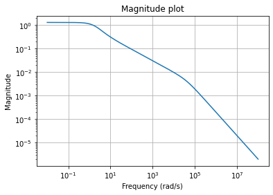
Note that mag_plot computes the
Frobenius norm of \(H(\boldsymbol{\imath} \omega)\) by default, just as scipy.linalg.norm.
Likewise, the choice of the norm \(\lVert \cdot \rVert\) can be controlled
using the ord parameter.
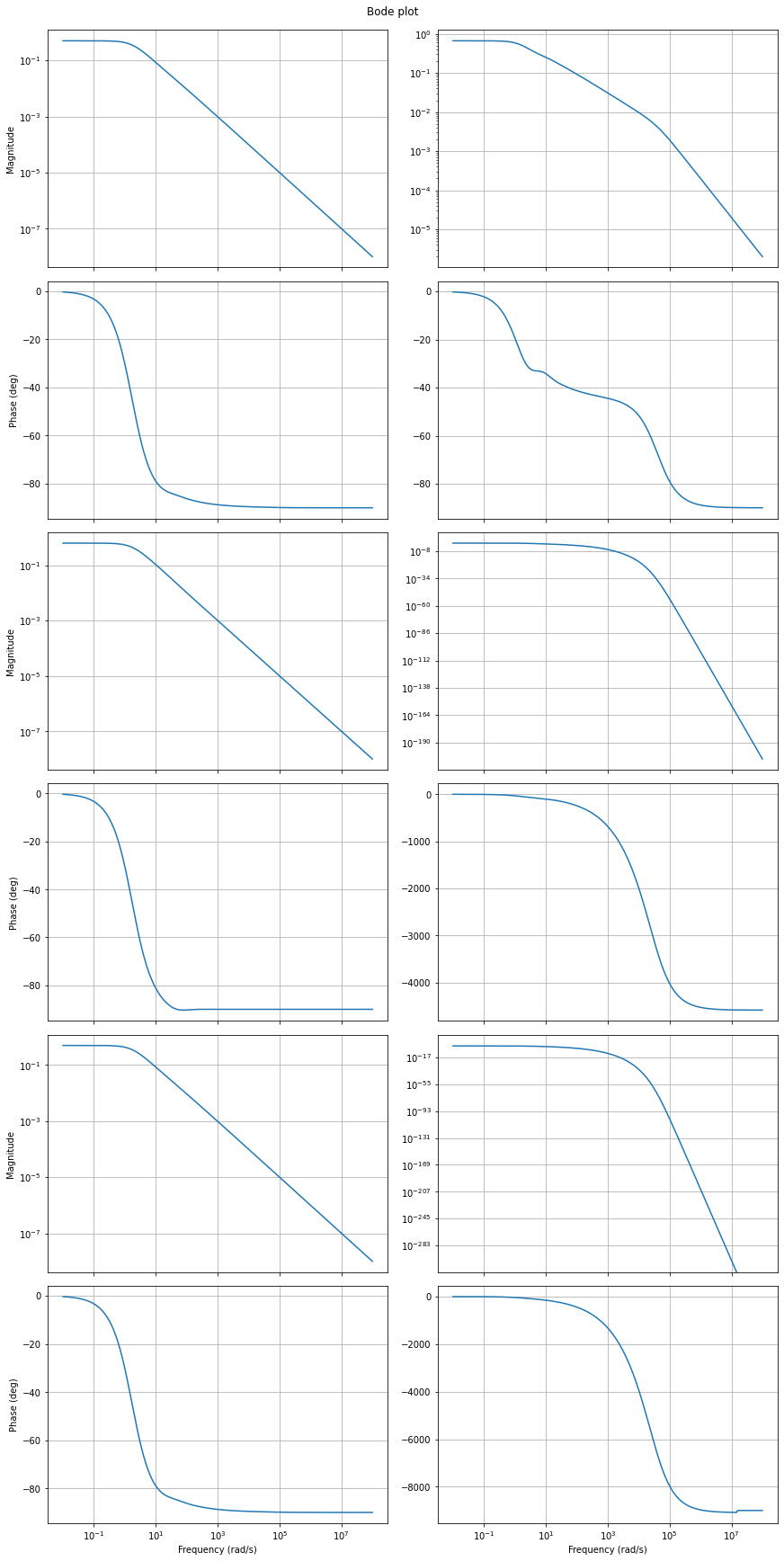
Another visualization is the Bode plot, which shows the magnitude and phase of each component of the transfer function. More specifically, \(\omega \mapsto \lvert H_{ij}(\boldsymbol{\imath} \omega) \rvert\) is in subplot \((2 i - 1, j)\) and \(\omega \mapsto \arg(H_{ij}(\boldsymbol{\imath} \omega))\) is in subplot \((2 i, j)\).
_ = fom.bode_plot(w)
System poles
The poles of an LTI system are the poles of its transfer function. From the form of the transfer function it follows that the poles are eigenvalues of \(E^{-1} A\), assuming that \(E\) is invertible. Conversely, the eigenvalues of \(E^{-1} A\) are the poles of the system in the generic case (more precisely, if the system is minimal, i.e., controllable and observable; see [A05]).
The poles of an LTIModel can be obtained using its
poles method
(assuming the system is minimal).
poles = fom.poles()
fig, ax = plt.subplots()
ax.plot(poles.real, poles.imag, '.')
_ = ax.set_title('Poles')
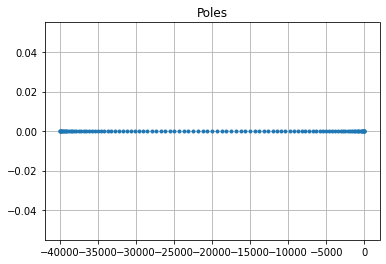
Note
The poles method uses a dense
eigenvalue solver,
which is applicable only up to medium-sized problems.
System Gramians
The controllability and observability Gramians of an asymptotically stable system with invertible \(E\) are respectively
From this, it is clear that \(P\) and \(Q\) are symmetric positive semidefinite. Furthermore, it can be shown that \(P\) and \(Q\) are solutions to Lyapunov equation
The Gramians can be used to quantify how much does the input influence the state (controllability) and state the output (observability). This is used to motivate the balanced truncation method (see Tutorial: Reducing an LTI system using balanced truncation). Also, they can be used to compute the \(\mathcal{H}_2\) norm (see below).
To find the “Gramians” \(P\) and \(Q\) of an LTIModel,
the gramian method can be used.
Although solutions to Lyapunov equations are generally dense matrices,
they can be often be very well approximated by a low-rank matrix.
With gramian,
it is possible to compute the dense solution of only the low-rank Cholesky
factor.
For example, the following computes the low-rank Cholesky factor of the
controllability Gramian as a VectorArray:
fom.gramian('c_lrcf')
NumpyVectorArray(
    [[-9.67050759e-01 -9.49603788e-01 -9.37818152e-01 ... -5.08356138e-01
      -5.03442167e-01 -4.98481264e-01]
     [-1.13133419e+00 -9.59580542e-01 -8.43810516e-01 ...  1.94699113e-01
       1.92880555e-01  1.91000976e-01]
     [ 9.08538963e-01  4.58145972e-01  2.24375612e-01 ...  9.25753046e-02
       9.17614570e-02  9.08841977e-02]
     ...
     [-4.48720858e-17  1.95466800e-15 -3.87392910e-14 ... -1.84179333e-10
       3.10420349e-11 -2.87160762e-12]
     [ 3.97648476e-18 -1.92190365e-16  4.26024322e-15 ... -2.24465928e-11
       1.75879252e-12 -8.24288506e-14]
     [-1.85127015e-17  7.70480426e-16 -1.45373940e-14 ...  1.65200046e-10
      -3.71100064e-11  4.41382006e-12]],
    NumpyVectorSpace(101, id='STATE'))
Hankel singular values
The Hankel singular values of an LTI system are \(\sigma_i = \sqrt{\lambda_i(E^{\operatorname{T}} Q E P)}\), where \(\lambda_i\) is the \(i\)-th eigenvalue.
Plotting the Hankel singular values shows us how well an LTI system can be
approximated by a reduced-order model.
The hsv method can be used to compute them.
hsv = fom.hsv()
fig, ax = plt.subplots()
ax.semilogy(range(1, len(hsv) + 1), hsv, '.-')
_ = ax.set_title('Hankel singular values')
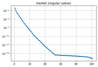
As expected for a heat equation, the Hankel singular values decay rapidly.
System norms
There are various system norms, used for quantifying the sensitivity of system’s outputs to its inputs. pyMOR currently has methods for computing: the \(\mathcal{H}_2\) norm, the \(\mathcal{H}_\infty\) norm, and the Hankel (semi)norm.
\(\mathcal{H}_2\) norm
The \(\mathcal{H}_2\) norm is (if \(E\) is invertible, \(E^{-1} A\) has eigenvalues in the open left half plane, and \(D\) is zero)
It can be shown that
Additionally, for systems with a single input or a single output (i.e., \(u(t) \in \mathbb{R}\) or \(y(t) \in \mathbb{R}\)),
The computation of the \(\mathcal{H}_2\) norm is based on the system Gramians
The h2_norm method of an LTIModel can be
used to compute it.
fom.h2_norm()
2.0377751533822073
\(\mathcal{H}_\infty\) norm
The \(\mathcal{H}_\infty\) norm is (if \(E\) is invertible and \(E^{-1} A\) has eigenvalues in the open left half plane)
It is always true that
and, in particular,
The hinf_norm method uses a dense solver
from Slycot to compute the
\(\mathcal{H}_\infty\) norm.
fom.hinf_norm()
1.2890705455704852
Hankel norm
The Hankel norm is (if \(E\) is invertible and \(E^{-1} A\) has eigenvalues in the open left half plane)
i.e., the largest Hankel singular value. Since it is independent of \(D\), the “Hankel norm” is only a seminorm in general.
It can be shown that the Hankel norm is the norm of the Hankel operator \(\mathcal{H} \colon \mathcal{L}_2(-\infty, 0) \to \mathcal{L}_2(0, \infty)\) mapping past inputs \(u_-\) to future outputs \(y_+\)
where \(h\) is the impulse response \(h(t) = C e^{t E^{-1} A} E^{-1} B + D \delta(t)\) (i.e., \(H\) is the Laplace transform of \(h\)). Thus,
The computation of the Hankel norm in
hankel_norm relies on the
hsv method.
fom.hankel_norm()
0.6221361786735345
Download the code:
tutorial_lti_systems.py,
tutorial_lti_systems.ipynb.