Tutorial: Model order reduction with artificial neural networks
Run this tutorial
Click here to run this tutorial on mybinder.org:Recent success of artificial neural networks led to the development of several methods for model order reduction using neural networks. pyMOR provides the functionality for a simple approach developed by Hesthaven and Ubbiali in [HU18]. For training and evaluation of the neural networks, PyTorch is used.
In this tutorial we will learn about feedforward neural networks, the basic idea of the approach by Hesthaven et al., and how to use it in pyMOR.
Feedforward neural networks
We aim at approximating a mapping \(h\colon\mathcal{P}\rightarrow Y\) between some input space \(\mathcal{P}\subset\mathbb{R}^p\) (in our case the parameter space) and an output space \(Y\subset\mathbb{R}^m\) (in our case the reduced space), given a set \(S=\{(\mu_i,h(\mu_i))\in\mathcal{P}\times Y: i=1,\dots,N\}\) of samples, by means of an artificial neural network. In this context, neural networks serve as a special class of functions that are able to “learn” the underlying structure of the sample set \(S\) by adjusting their weights. More precisely, feedforward neural networks consist of several layers, each comprising a set of neurons that are connected to neurons in adjacent layers. A so called “weight” is assigned to each of those connections. The weights in the neural network can be adjusted while fitting the neural network to the given sample set. For a given input \(\mu\in\mathcal{P}\), the weights between the input layer and the first hidden layer (the one after the input layer) are multiplied with the respective values in \(\mu\) and summed up. Subsequently, a so called “bias” (also adjustable during training) is added and the result is assigned to the corresponding neuron in the first hidden layer. Before passing those values to the following layer, a (non-linear) activation function \(\rho\colon\mathbb{R}\rightarrow\mathbb{R}\) is applied. If \(\rho\) is linear, the function implemented by the neural network is affine, since solely affine operations were performed. Hence, one usually chooses a non-linear activation function to introduce non-linearity in the neural network and thus increase its approximation capability. In some sense, the input \(\mu\) is passed through the neural network, affine-linearly combined with the other inputs and non-linearly transformed. These steps are repeated in several layers.
The following figure shows a simple example of a neural network with two hidden layers, an input size of two and an output size of three. Each edge between neurons has a corresponding weight that is learnable in the training phase.
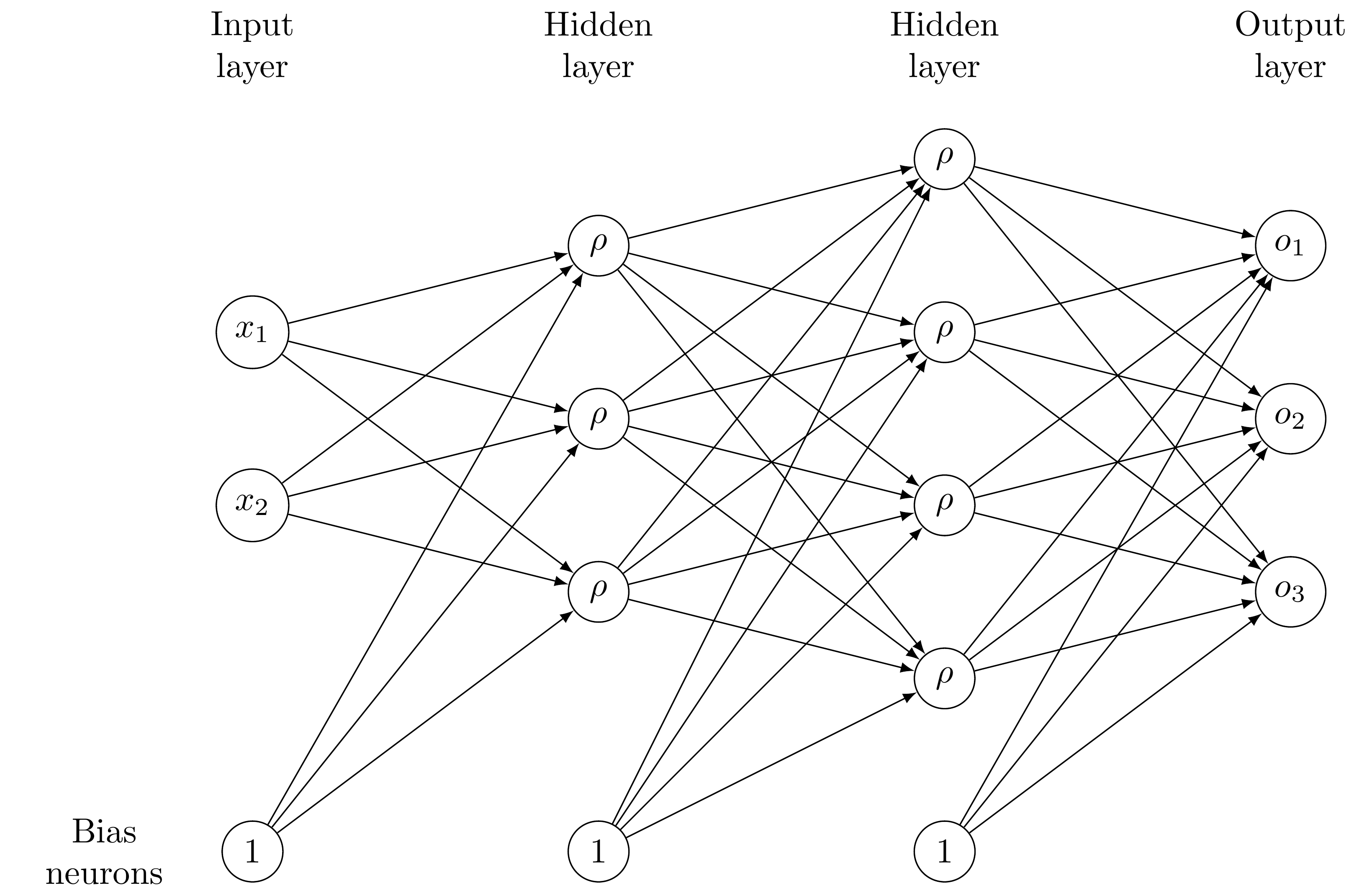
To train the neural network, one considers a so called “loss function”, that measures how the neural network performs on the training set \(S\), i.e. how accurately the neural network reproduces the output \(h(\mu_i)\) given the input \(\mu_i\). The weights of the neural network are adjusted iteratively such that the loss function is successively minimized. To this end, one typically uses a Quasi-Newton method for small neural networks or a (stochastic) gradient descent method for deep neural networks (those with many hidden layers).
A possibility to use feedforward neural networks in combination with reduced basis methods will be introduced in the following section.
A non-intrusive reduced order method using artificial neural networks
We now assume that we are given a parametric pyMOR Model for which we want
to compute a reduced order surrogate Model using a neural network. In this
example, we consider the following two-dimensional diffusion problem with
parametrized diffusion, right hand side and Dirichlet boundary condition:
on the domain \(\Omega:= (0, 1)^2 \subset \mathbb{R}^2\) with data functions \(f((x_1, x_2), \mu) = 10 \cdot \mu + 0.1\), \(\sigma((x_1, x_2), \mu) = (1 - x_1) \cdot \mu + x_1\), where \(\mu \in (0.1, 1)\) denotes the parameter. Further, we apply the Dirichlet boundary conditions
We discretize the problem using pyMOR’s builtin discretization toolkit as explained in Tutorial: Using pyMOR’s discretization toolkit:
from pymor.basic import *

problem = StationaryProblem(
      domain=RectDomain(),

      rhs=LincombFunction(
          [ExpressionFunction('ones(x.shape[:-1]) * 10', 2, ()), ConstantFunction(1., 2)],
          [ProjectionParameterFunctional('mu'), 0.1]),

      diffusion=LincombFunction(
          [ExpressionFunction('1 - x[..., 0]', 2, ()), ExpressionFunction('x[..., 0]', 2, ())],
          [ProjectionParameterFunctional('mu'), 1]),

      dirichlet_data=LincombFunction(
          [ExpressionFunction('2 * x[..., 0]', 2, ()), ConstantFunction(1., 2)],
          [ProjectionParameterFunctional('mu'), 0.5]),

      name='2DProblem'
  )

fom, _ = discretize_stationary_cg(problem, diameter=1/50)
Since we employ a single Parameter, and thus use the same range for each
parameter, we can create the ParameterSpace using the following line:
parameter_space = fom.parameters.space((0.1, 1))
The main idea of the approach by Hesthaven et al. is to approximate the mapping
from the Parameters to the coefficients of the respective solution in a
reduced basis by means of a neural network. Thus, in the online phase, one
performs a forward pass of the Parameters through the neural networks and
obtains the approximated reduced coordinates. To derive the corresponding
high-fidelity solution, one can further use the reduced basis and compute the
linear combination defined by the reduced coefficients. The reduced basis is
created via POD.
The method described above is “non-intrusive”, which means that no deep insight into the model or its implementation is required and it is completely sufficient to be able to generate full order snapshots for a randomly chosen set of parameters. This is one of the main advantages of the proposed approach, since one can simply train a neural network, check its performance and resort to a different method if the neural network does not provide proper approximation results.
In pyMOR, there exists a training routine for feedforward neural networks. This procedure is part of a reductor and it is not necessary to write a custom training algorithm for each specific problem. However, it is sometimes necessary to try different architectures for the neural network to find the one that best fits the problem at hand. In the reductor, one can easily adjust the number of layers and the number of neurons in each hidden layer, for instance. Furthermore, it is also possible to change the deployed activation function.
To train the neural network, we create a training and a validation set
consisting of 100 and 20 randomly chosen parameter values, respectively:
training_set = parameter_space.sample_uniformly(100)
validation_set = parameter_space.sample_randomly(20)
In this tutorial, we construct the reduced basis such that no more modes than
required to bound the l2-approximation error by a given value are used.
The l2-approximation error is the error of the orthogonal projection (in the
l2-sense) of the training snapshots onto the reduced basis. That is, we
prescribe l2_err in the reductor. It is also possible to determine a relative
or absolute tolerance (in the singular values) that should not be exceeded on
the training set. Further, one can preset the size of the reduced basis.
The training is aborted when a neural network that guarantees our prescribed
tolerance is found. If we set ann_mse to None, this function will
automatically train several neural networks with different initial weights and
select the one leading to the best results on the validation set. We can also
set ann_mse to 'like_basis'. Then, the algorithm tries to train a neural
network that leads to a mean squared error on the training set that is as small
as the error of the reduced basis. If the maximal number of restarts is reached
without finding a network that fulfills the tolerances, an exception is raised.
In such a case, one could try to change the architecture of the neural network
or switch to ann_mse=None which is guaranteed to produce a reduced order
model (perhaps with insufficient approximation properties).
We can now construct a reductor with prescribed error for the basis and mean squared error of the neural network:
from pymor.reductors.neural_network import NeuralNetworkReductor

reductor = NeuralNetworkReductor(fom,
                                 training_set,
                                 validation_set,
                                 l2_err=1e-5,
                                 ann_mse=1e-5)
To reduce the model, i.e. compute a reduced basis via POD and train the neural
network, we use the respective function of the
NeuralNetworkReductor:
rom = reductor.reduce(restarts=100)
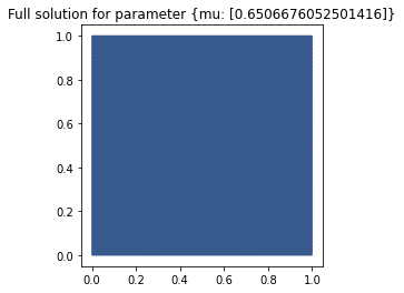
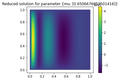
We are now ready to test our reduced model by solving for a random parameter value the full problem and the reduced model and visualize the result:
mu = parameter_space.sample_randomly(1)[0]

U = fom.solve(mu)
U_red = rom.solve(mu)
U_red_recon = reductor.reconstruct(U_red)

fom.visualize((U, U_red_recon),
              legend=(f'Full solution for parameter {mu}', f'Reduced solution for parameter {mu}'))
Finally, we measure the error of our neural network and the performance
compared to the solution of the full order problem on a training set. To this
end, we sample randomly some parameter values from our ParameterSpace:
test_set = parameter_space.sample_randomly(10)
Next, we create empty solution arrays for the full and reduced solutions and an empty list for the speedups:
U = fom.solution_space.empty(reserve=len(test_set))
U_red = fom.solution_space.empty(reserve=len(test_set))

speedups = []
Now, we iterate over the test set, compute full and reduced solutions to the respective parameters and measure the speedup:
import time

for mu in test_set:
    tic = time.perf_counter()
    U.append(fom.solve(mu))
    time_fom = time.perf_counter() - tic

    tic = time.perf_counter()
    U_red.append(reductor.reconstruct(rom.solve(mu)))
    time_red = time.perf_counter() - tic

    speedups.append(time_fom / time_red)
We can now derive the absolute and relative errors on the training set as
absolute_errors = (U - U_red).norm()
relative_errors = (U - U_red).norm() / U.norm()
The average absolute error amounts to
import numpy as np

np.average(absolute_errors)
7.666763166475745e+26
On the other hand, the average relative error is
np.average(relative_errors)
9.170277209546442e+24
Using neural networks results in the following median speedup compared to solving the full order problem:
np.median(speedups)
10.030416977344256
Since NeuralNetworkReductor only calls
the solve method of the Model, it can easily
be applied to Models originating from external solvers, without requiring any access to
Operators internal to the solver.
Download the code:
tutorial_mor_with_anns.py
tutorial_mor_with_anns.ipynb